Next: Model
Assessment Previous: Rules:
Sources of Mortality
In the unscaled model estuary, a density of 0.1 crabs/m![]() represents
represents
![]() crabs. Although parallel computers make it possible to model this
number of crabs, a reduction in the computational demands can be
achieved by scaling the estuary. In scaling down the size of the
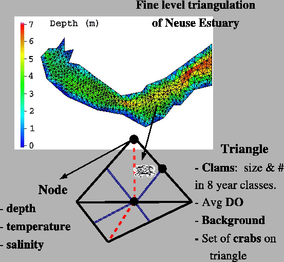
estuary, two things are considered. First, the size of the fine-level
triangles (Appendix A.3)
must be sufficiently small to provide the degree of spatial
resolution required to observe desired changes in the spatial
distribution of crabs, clams and background prey. Secondly, the
number of crabs in the estuary must be sufficiently large that the
probability of a fine-level triangle being unoccupied by chance is
small. These two criteria work against each other. On the one hand,
increasing the number of fine-level triangles (decreasing their size
or area) will lead to greater spatial resolution in clam and
background biomass distribution. Alternatively, if the number of
crabs in the estuary is kept constant, increasing the number of
fine-level triangles will increase the spatial variability in crab
density and biomass since there will be a greater chance that each
triangle contains none or only a single crab.
crabs. Although parallel computers make it possible to model this
number of crabs, a reduction in the computational demands can be
achieved by scaling the estuary. In scaling down the size of the
estuary, two things are considered. First, the size of the fine-level
triangles (Appendix A.3)
must be sufficiently small to provide the degree of spatial
resolution required to observe desired changes in the spatial
distribution of crabs, clams and background prey. Secondly, the
number of crabs in the estuary must be sufficiently large that the
probability of a fine-level triangle being unoccupied by chance is
small. These two criteria work against each other. On the one hand,
increasing the number of fine-level triangles (decreasing their size
or area) will lead to greater spatial resolution in clam and
background biomass distribution. Alternatively, if the number of
crabs in the estuary is kept constant, increasing the number of
fine-level triangles will increase the spatial variability in crab
density and biomass since there will be a greater chance that each
triangle contains none or only a single crab.
The number of refinement levels and average unscaled area of the
triangles were listed in Appendix A.3
with the finest level consisting of 1079 triangles. Based on a
uniform distribution of crabs over the estuary,
![]() 2000 crabs are required to ensure that the chance of a triangle being
empty by chance is less than 20%. The dimensions of the estuary are
scaled by a factor of 100 so that the area of the scaled estuary
becomes
2000 crabs are required to ensure that the chance of a triangle being
empty by chance is less than 20%. The dimensions of the estuary are
scaled by a factor of 100 so that the area of the scaled estuary
becomes
![]() m
m![]() and 2000 crabs corresponds to an average crab density of
and 2000 crabs corresponds to an average crab density of
![]() crabs/m
crabs/m![]() .
Thus, in the scaled estuary each individual crab can be thought of as
representing a cohort of similar crabs (say in size and spatial
location) in the unscaled estuary. Provided one does not aggregate to
the extremes, the behavior of individuals in the scaled estuary will
adequately represent the behaviors occurring in the unscaled estuary.
Given that the scaled estuary is a miniature model of the unscaled
estuary, we also scale down the velocity at which crabs move and the
maximum interaction distance over which crabs interact. In
this way, it is as if the crabs in the scaled estuary are moving
about with similar probabilities of encountering each other or the
estuary boundary as in the unscaled estuary. However, each crab's
energy usage is calculated as if it were moving about at the unscaled
rates of movement.
.
Thus, in the scaled estuary each individual crab can be thought of as
representing a cohort of similar crabs (say in size and spatial
location) in the unscaled estuary. Provided one does not aggregate to
the extremes, the behavior of individuals in the scaled estuary will
adequately represent the behaviors occurring in the unscaled estuary.
Given that the scaled estuary is a miniature model of the unscaled
estuary, we also scale down the velocity at which crabs move and the
maximum interaction distance over which crabs interact. In
this way, it is as if the crabs in the scaled estuary are moving
about with similar probabilities of encountering each other or the
estuary boundary as in the unscaled estuary. However, each crab's
energy usage is calculated as if it were moving about at the unscaled
rates of movement.
|
|
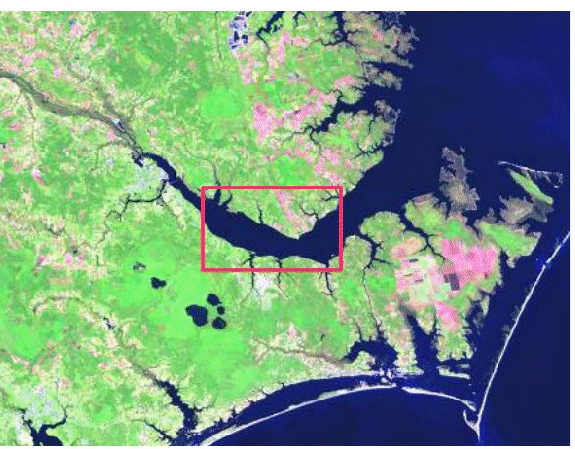
| FIG. A2. The Neuse River originates north of Durham, NC has a watershed area of 16,102 km |
|
|
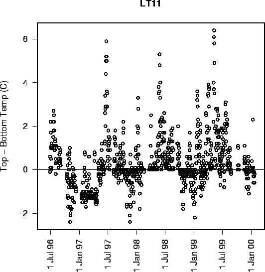
FIG. A3. Plot of daily differences in top and bottom water temperatures from site LT11 in the Neuse River Estuary. Data from USGS. |
|
|
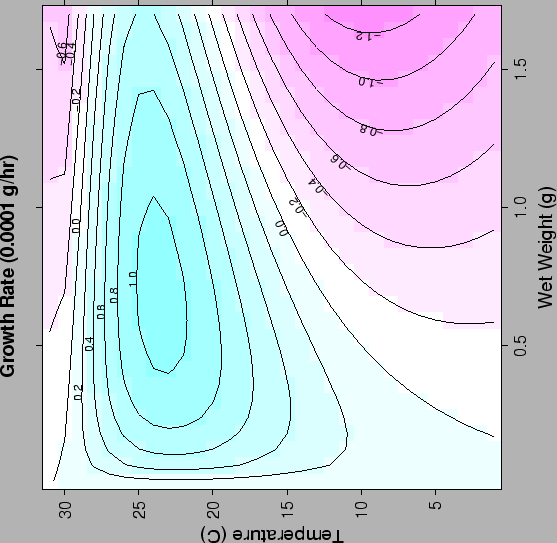
| FIG. A4. Clam growth rate at a given mass and temperature for DO |
|
|
|
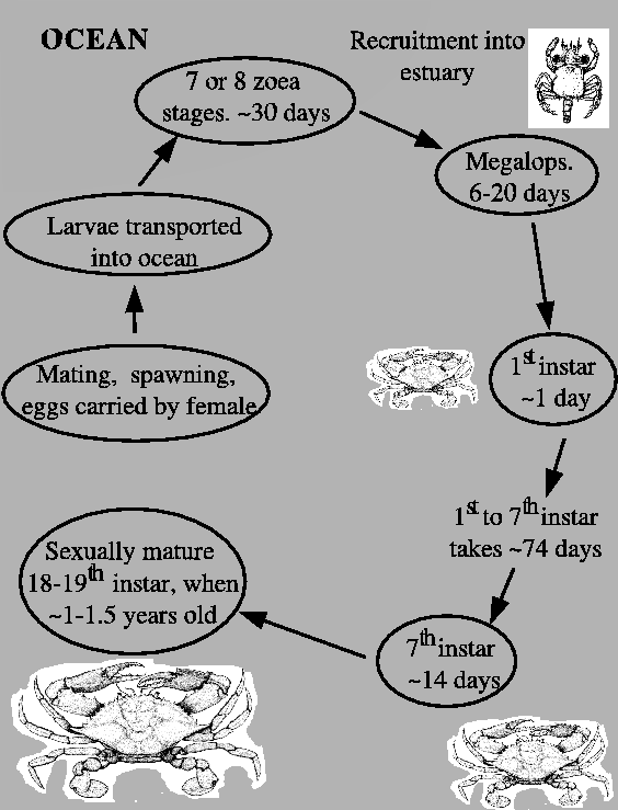
FIG. A5. The blue crab has a complex life-cycle. The zoea stages are spent in the ocean. Megalops are recruited back into the estuary where crabs spend the rest of their lives. The body plan of an adult crab is evident upon reaching the first instar. |
|
|
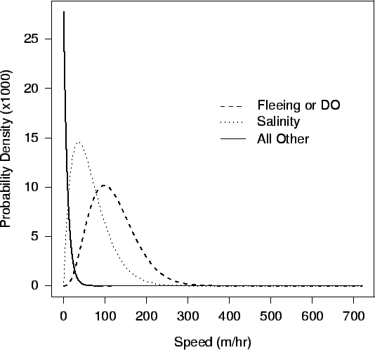
| FIG. A6. Movement distribution for a 200 g crab at a temperature of
|
|
|
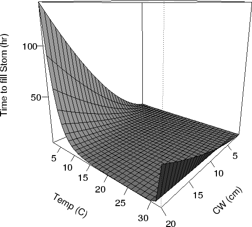
FIG. A7. Time for a completely empty crab stomach to fill due to ingestion as a function of CW (cm) and temperature (
|
|
|
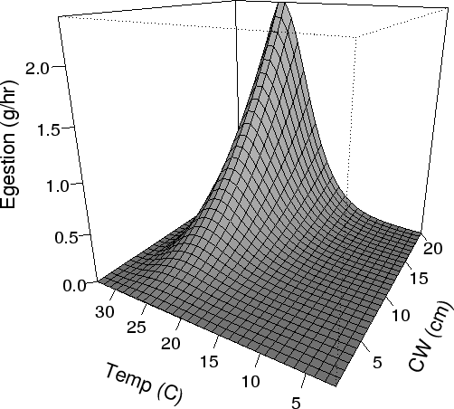
| FIG. A8. Rate of egestion (g/hr) from the stomach of different sized crabs vs temperature (Eqn A.40). |
|
|
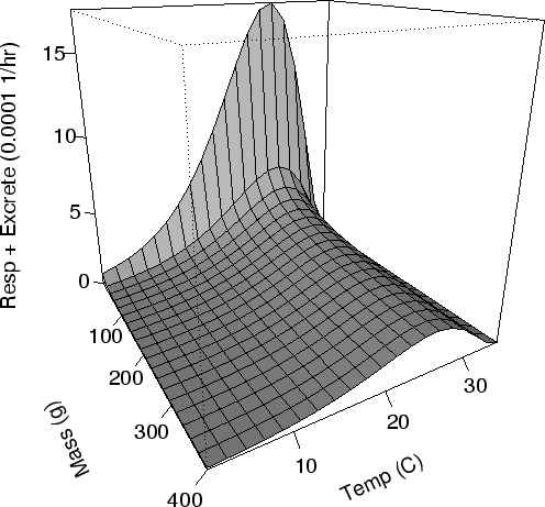
| FIG. A9. Energy usage per g of crab mass ( |
|
|
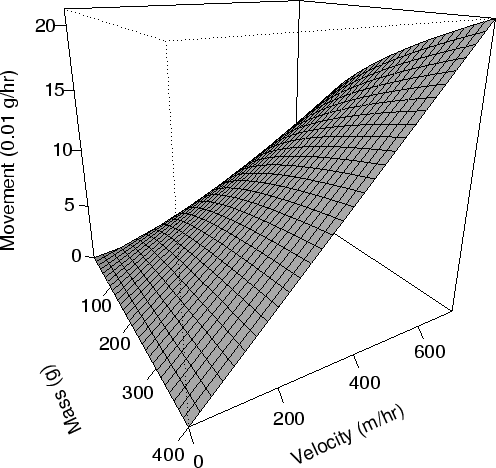
| FIG. A.10. Energy usage in grams per mass of crab (0.01 g/hr) for crabs moving at different velocities (Eqn A.45). |
|
|
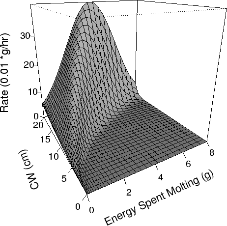
| FIG. A11. Rate (0.01 g/hr) at which crabs expend energy as they molt as a function of the total energy required to molt (g) and the CW (cm) of the crab. Temperature is at
|
Next: Model
Assessment Previous: Rules:
Sources of Mortality