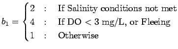
Many crustaceans are tolerant of hypoxic exposure and can regulate oxygen consumption at low oxygen concentrations (McMahon 2001). However, both the impacts of hypoxia and a crab's reaction to it are stage specific. Adult crabs avoid hypoxic water (Das and Stickle 1994; Lowery and Tate 1986; Pihl et al. 1991). Juvenile crabs (20-25 mm carapace width, CW) prefer oxygen concentrations of 4.5 to 5.8 mg/L, but have a reduced ability to detect low oxygen and to find and remain in optimal oxygen conditions (Das and Stickle 1994). Crabs exposed to normoxia grow faster, have a higher feeding rate, molt more and have a shorter intermolt interval than those exposed to low oxygen conditions (Das and Stickle 1993). Adult males tend to spend their lives in lower salinity water located in the upper part of the estuary. Prior to mating, females are distributed throughout the estuary, but following mating remain in higher salinity waters near the mouth of the estuary.
Individual crabs in this model are assumed to be moving continuously
with a rate, ![]() (m/hr), at an angle
(m/hr), at an angle
![]() relative to the horizontal axis of the estuary. Movement is
determined by the crab's local environment or the finest level
triangle containing the crab. Since crabs move continuously in space,
determining this fine level triangle is accomplished using the nested
conforming triangulation of the estuary
(Fig. A1). After determining the coarsest-level
triangle containing the crab with an iterative search, one then
searches within the triangles that each coarser level triangle is
divided into (Fig. A1) and one repeats this
process down the nested triangulation levels. The average
computational cost of finding the finest-level triangle containing the
crab using such an algorithm is much less than if we were to
exhaustively search over all finest-level triangles. Such nested
triangulations also play a central role in adaptive multigrid
algorithms used to numerically solve partial differential
equations (e.g., Braess 1997) and will be useful if more
detailed and mathematically complex models (e.g., a partial
differential equation model for DO) are ever required.
relative to the horizontal axis of the estuary. Movement is
determined by the crab's local environment or the finest level
triangle containing the crab. Since crabs move continuously in space,
determining this fine level triangle is accomplished using the nested
conforming triangulation of the estuary
(Fig. A1). After determining the coarsest-level
triangle containing the crab with an iterative search, one then
searches within the triangles that each coarser level triangle is
divided into (Fig. A1) and one repeats this
process down the nested triangulation levels. The average
computational cost of finding the finest-level triangle containing the
crab using such an algorithm is much less than if we were to
exhaustively search over all finest-level triangles. Such nested
triangulations also play a central role in adaptive multigrid
algorithms used to numerically solve partial differential
equations (e.g., Braess 1997) and will be useful if more
detailed and mathematically complex models (e.g., a partial
differential equation model for DO) are ever required.
Unlike the above algorithm, movement of individuals in IBMs is typically done by dividing the spatial domain into small cells with individuals moving between neighboring cells when updated. Such movement algorithms, however, have limitations relative to the one outlined above (Tischendorf 1997). First, the size of the grid is limited by memory capacity and computational time required to iterate over the entire grid. Second, the fixed spatial structure implies equal resolution for both landscape features and individual movements. Finally, individuals can only move in complete cell units and are limited in movement angles. For such a movement algorithm to work, the distance between cells must be small relative to the individual's actual movement rates and a balance must be found between computational tractability (number of cells that can be stored in memory) and the time resolution of the model. The smaller each individual cell, the smaller the time resolution over which the model can be advanced, but the greater the model's computational demands.
The crab's new direction of movement,
![]() , is arrived
at by generating a new random change in direction based on a variety
of factors, including oxygen concentration, salinity, depth, whether
the crab is fleeing as a result of an interaction or if the crab has
hit the boundary of the estuary.
, is arrived
at by generating a new random change in direction based on a variety
of factors, including oxygen concentration, salinity, depth, whether
the crab is fleeing as a result of an interaction or if the crab has
hit the boundary of the estuary.
![]() is kept with
is kept with
![]() .
.
If the crab is not fleeing and it has not hit the
estuary boundary, then
![]() is generated randomly
based on trying to maximize or minimize environment variables. The
environment variables are not all of equal importance in determining a
crab's direction of motion. In the list below, conditions further
down in the list over-ride earlier ones. Let
is generated randomly
based on trying to maximize or minimize environment variables. The
environment variables are not all of equal importance in determining a
crab's direction of motion. In the list below, conditions further
down in the list over-ride earlier ones. Let ![]() denote a
realization of a uniform random variable generated over the interval
denote a
realization of a uniform random variable generated over the interval
![]() and let
and let ![]() denote the current
direction of the crab. Let
denote the current
direction of the crab. Let ![]() denote the direction in which
the particular environment variable is maximum/minimum (depending on
the context) and is computed based on the values of the variable at
the three nodes defining the triangle of the crab's current triangle
in the case of salinity and depth and using the neighboring set of
triangles for DO.
denote the direction in which
the particular environment variable is maximum/minimum (depending on
the context) and is computed based on the values of the variable at
the three nodes defining the triangle of the crab's current triangle
in the case of salinity and depth and using the neighboring set of
triangles for DO.
A crab's maximum rate of movement,
![]() , for a 200 g crab
is
, for a 200 g crab
is
![]() (m/hr) (Wolcott and Hines 1990; Houlihan et al. 1985; Clark et al. 1999). In
the model, the maximum rate of movement decreases with decreasing crab
size. The new rate of crab movement,
(m/hr) (Wolcott and Hines 1990; Houlihan et al. 1985; Clark et al. 1999). In
the model, the maximum rate of movement decreases with decreasing crab
size. The new rate of crab movement, ![]() (m/hr), depends on whether
the crab is eating or molting, the temperature of the crab's
environment, whether the crab has lost weight because it is starved,
whether it is fleeing from another crab, moving out of an hypoxic
patch, or moving away from or into higher or lower salinity water.
The factor decrease in the crab's maximum rate of movement,
(m/hr), depends on whether
the crab is eating or molting, the temperature of the crab's
environment, whether the crab has lost weight because it is starved,
whether it is fleeing from another crab, moving out of an hypoxic
patch, or moving away from or into higher or lower salinity water.
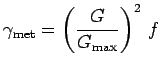
The factor decrease in the crab's maximum rate of movement,
![]() , depends on how the temperature of the crab's
environment differs from
, depends on how the temperature of the crab's
environment differs from
![]() and whether the crab
lost weight due to starvation:
and whether the crab
lost weight due to starvation:
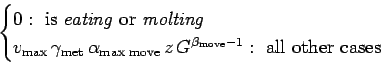
Let
![]() (g
(g
![]() ). The actual rate of crab movement,
). The actual rate of crab movement, ![]() (m/hr),
depends on whether the crab is eating or molting and environmental
conditions:
(m/hr),
depends on whether the crab is eating or molting and environmental
conditions: