Crabs are highly cannibalistic with large crabs (14-16 cm carapace
width) accounting for very high rates of juvenile mortality (40-90%
in Chesapeake Hines and Ruiz (1995), ![]() 85% in
Alabama Spitzer et al. (2003)), with somewhat lower rates farther
north (Heck Jr and Coen 1995). Juvenile crabs in turn prey on smaller
crabs and megalopae (Moksnes et al. 1997). A variety of fish and
birds are also known to consume blue crab, but in insignificant
numbers relative to larger crabs (Hines, in press; Hines and Ruiz 1995).
Blue crabs engage in aggressive and defensive behaviors to fend off
other crabs from food or mates. In tank experiments, such behaviors
occurred when two crabs were within 10 cm of each other (Jachowski 1974). Larger individuals almost always dominate
smaller ones (Dittel et al. 1995) and males typically dominate
females (Jachowski 1974). Many invertebrate and vertebrate
species respond to threat or injury by autotomizing an
appendage. Approximately 25% and 18% of the crabs sampled from
Chesapeake Bay in 1986 and 1987, respectively, were missing one or
more limbs, usually a cheliped (Smith 1990). We do not model
autotomy because limited levels of autotomy do not appear to alter
crab behaviors (Jachowski 1974) or life history
(Smith and Hines 1991; Smith 1995).
85% in
Alabama Spitzer et al. (2003)), with somewhat lower rates farther
north (Heck Jr and Coen 1995). Juvenile crabs in turn prey on smaller
crabs and megalopae (Moksnes et al. 1997). A variety of fish and
birds are also known to consume blue crab, but in insignificant
numbers relative to larger crabs (Hines, in press; Hines and Ruiz 1995).
Blue crabs engage in aggressive and defensive behaviors to fend off
other crabs from food or mates. In tank experiments, such behaviors
occurred when two crabs were within 10 cm of each other (Jachowski 1974). Larger individuals almost always dominate
smaller ones (Dittel et al. 1995) and males typically dominate
females (Jachowski 1974). Many invertebrate and vertebrate
species respond to threat or injury by autotomizing an
appendage. Approximately 25% and 18% of the crabs sampled from
Chesapeake Bay in 1986 and 1987, respectively, were missing one or
more limbs, usually a cheliped (Smith 1990). We do not model
autotomy because limited levels of autotomy do not appear to alter
crab behaviors (Jachowski 1974) or life history
(Smith and Hines 1991; Smith 1995).
In the model, we assume that a potential interacting crab can be
chosen randomly based on the distance between the crab being updated
and neighboring crabs. The set of neighboring crabs is found by
aggregating the crabs located on the neighboring fine-level triangles
within
![]() max inter=12 m (the max interaction
distance) of the crab being updated. Crabs that are further than
max inter=12 m (the max interaction
distance) of the crab being updated. Crabs that are further than
![]() apart are assumed not to interact. Each crab
stores the last crab it interacted with and this crab is excluded from
the set of possible interactions. The distance between each
neighboring crab,
apart are assumed not to interact. Each crab
stores the last crab it interacted with and this crab is excluded from
the set of possible interactions. The distance between each
neighboring crab, ![]() , and the crab being updated,
, and the crab being updated,
![]() , is computed and
, is computed and ![]() is randomly designated as a
potential interacting crab if
is randomly designated as a
potential interacting crab if
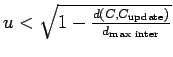 where
where ![]() is a realization
of a uniform random variable on
is a realization
of a uniform random variable on ![]() . The potential interaction
time of these two crabs is generated randomly over the smallest time
interval until either crab was scheduled to be updated again
(Appendix A.5.2). Over all potential
interaction times, the pair of potentially interacting crabs with the
smallest randomly generated update time is stored in the
priority queue and in each crab's interaction set.
As a result, crabs that are closer to each other have a greater chance
of interacting.
. The potential interaction
time of these two crabs is generated randomly over the smallest time
interval until either crab was scheduled to be updated again
(Appendix A.5.2). Over all potential
interaction times, the pair of potentially interacting crabs with the
smallest randomly generated update time is stored in the
priority queue and in each crab's interaction set.
As a result, crabs that are closer to each other have a greater chance
of interacting.
A scheduled interaction will not occur if one of the crabs is updated because of an earlier scheduled update. If the interaction does occur, possible outcomes include that nothing happens to either crab, one crab is killed and nothing happens to the other, or one crab flees while nothing happens to the other. The actual outcome of the interaction depends on a large number of factors: gut fullness, whether one or both crabs are molting, the sexes of the interacting crabs, whether an interacting female is in her final molt, and the size difference between the crabs. The rules governing the outcome of interactions are not complex, but many different cases must be considered. These interaction rules are given below. A killed crab becomes food for the crab that killed it. If a feeding crab flees, its mass of food feeding on (Appendix A.5.6) is passed off to the attacking crab.
The interaction rules between two crabs, A and B are symmetric and so will only be described relative to Crab A. If the crabs are both molting, nothing happens to either of them. If crab A is molting then:
Finally, we discuss the case when both crabs are not molting. The
idea behind this rule is that crabs only attack other crabs and
kill/eat them if their gut is almost empty and there are particular
size differences between the two crabs. Let
![]() , where
, where ![]() is the
volume of food in the crab's stomach.
is the
volume of food in the crab's stomach. ![]() is between zero and 1 and
denotes ``gut emptiness''. Let
is between zero and 1 and
denotes ``gut emptiness''. Let ![]() ,
,
![]() and
and ![]() be a
realization of standard uniform random variable on
be a
realization of standard uniform random variable on ![]() . Let
. Let
![]() inter
inter![]() and
and
Then,
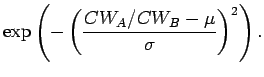
For
![]() for Crab A, if both crabs are the same size, then
there is only a small chance that B is killed. When A is twice as big
as B, B is killed with probability 0.8, and when A is 3 times as big
as B, B has a low probability of being killed since it is less likely
that A would bother with such small prey.
for Crab A, if both crabs are the same size, then
there is only a small chance that B is killed. When A is twice as big
as B, B is killed with probability 0.8, and when A is 3 times as big
as B, B has a low probability of being killed since it is less likely
that A would bother with such small prey.