Temperature

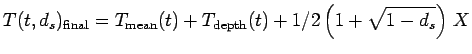
Bottom water temperatures in the Neuse range between 4 and 32$^\circ$ C (Borsuk et al. 2001b; Selberg et al. 2001). The temperature field consists of deterministic and random components and is given by:

$$T(t, d_s)_{\text{final}} = T_{\text{mean}}(t) + T_\text{depth}(t) + 1/2\left(1 +\sqrt{1-d_s}\right)\,X$$ (A.3)

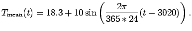
The first part of the temperature field is deterministic and was obtained by fitting time-series data of bottom water temperature from a single location in the Neuse (LT11 near the bend in Fig. A2). These data were fit to a sinusoidal function where time, $t$, is in hours:

$$T_{\text{mean}}(t) = 18.3 + 10\sin\left(\frac{2\pi}{365*24}(t - 3020)\right).$$ (A.4)

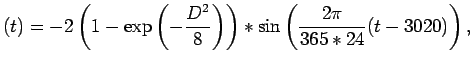
The second term in Eqn (A.3) alters $T_{\text{mean}}$ depending on the depth $D(x,y)$ at a given location $(x,y)$ and the season:

$$(t) = - 2\left(1-\exp\left(-\frac{D^2}{8}\right)\right)*\sin\left(\frac{2\pi}{365*24}(t - 3020)\right),$$ (A.5)

causing deeper areas to be slightly (up to 2 $\ensuremath{^\circ\text{C }}$) warmer in winter and colder in summer (the reverse for shallower areas) to reflect estuarine patterns (Fig. A3).

The Gaussian random field, $X$, in Eqn (A.3) is generated with $\sigma_{x, T}$, $\sigma_{y,T}$, and $\sigma_{t, T}$ set to 1000 (m), 800 (m) and 48 (hrs) respectively based on the data presented in Luettich Jr. et al. (1999) and Selberg et al. (2001). The degree of variation in the final field is assumed to decrease toward the eastern boundary of the estuary. Let $d_s = d(x, y)/d_$max be the proportional horizontal distance from the western most boundary of the estuary and $d_$max (m) the maximum horizontal length of the estuary. See the online appendices for movies and Appendix B.2 for further summary of this and the other environment variables.