The entire 2D model estuary is enclosed in a rectangle that is
discretized into a total of ![]() and
and ![]() points in the
points in the ![]() and
and ![]() directions, while the number of points used over the time interval
(March 16th to November 14th) is
directions, while the number of points used over the time interval
(March 16th to November 14th) is ![]() . This leads to a series of
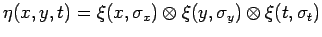
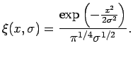
rectangles in space and time. Gaussian random fields are generated
over this rectangular grid using a FFT
algorithm (Dietrich and Newsam 1993) with filter:
. This leads to a series of
rectangles in space and time. Gaussian random fields are generated
over this rectangular grid using a FFT
algorithm (Dietrich and Newsam 1993) with filter:
 are not very correlated. The number of
discretization points (
are not very correlated. The number of
discretization points ( ,
,  and
and  ) are chosen so that
 for
for
 where
where
 is
the constant distance between discretization
points (Dietrich and Newsam 1993). The random fields are generated
independently each year for the 245 days between March 16 and November
14th. No randomness is present in these environment variables for the
remaining time period (November 15th to March 15) that the model runs
over. Because the temperature in the estuary is low during this
period, a crab's respiration and growth rates will also be low and the
lack of spatial heterogeneity in environmental variables will not
homogenize the crab population. Finally, the values of the generated
random field are interpolated from the rectangular grid onto the
finest triangulation of the estuary and exported to a file. As the
crab model runs, the appropriate values are read in every 24 hours.
Pre-generating these variables lessens the computational burden.
is
the constant distance between discretization
points (Dietrich and Newsam 1993). The random fields are generated
independently each year for the 245 days between March 16 and November
14th. No randomness is present in these environment variables for the
remaining time period (November 15th to March 15) that the model runs
over. Because the temperature in the estuary is low during this
period, a crab's respiration and growth rates will also be low and the
lack of spatial heterogeneity in environmental variables will not
homogenize the crab population. Finally, the values of the generated
random field are interpolated from the rectangular grid onto the
finest triangulation of the estuary and exported to a file. As the
crab model runs, the appropriate values are read in every 24 hours.
Pre-generating these variables lessens the computational burden.