Altering All Clam Factors Together

To assess the combined impact of all model changes for the cases above, the above changes were made jointly and clam density was decreased even further than in Appendix B.5.2. Clam biomass was originally 334 (g/m$^2$), (Table C2) while after the these modifications increased to 715 (g/m$^2$) even though clam density was decreased to 388 (#/m$^2$) compared to 893 (#/m$^2$) originally. The net result was that adult crab density increased to 0.0200 from 0.0145 (#/m$^2$). Crabs showed no evidence of food limitation (gut fullness $> 0.44$ for all instar classes and egg production per mature female was 2297 #/# hr). These values were all greater than those obtained under the original 45% Short case (Table C2). Thus, the combined effect of the misspecifications in the clam model for the Neuse River estuary had no effect on the larger conclusion reached - namely that crab population dynamics are primarily controlled by cannibalism and not food limitation.

   FIG. B1. The number of consecutive days locations remain hypoxic (DO $<$ 2 mg/L) under the model during years 18 and 19. 20 day consecutive non-overlapping windows are used. Results are shown for all fine-level triangles in the estuary, conditioned on depth and year.

 

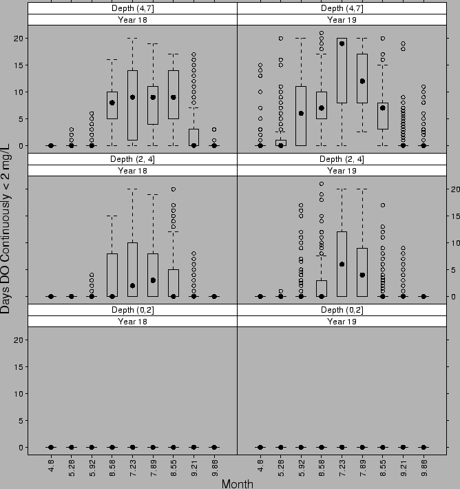
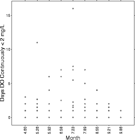
   FIG. B2. Durations of hypoxia (DO $<$ 2 mg/L) at measurement sites LT9 and LT11 in the Neuse over years 1989 to 1999. As in Fig. B1, durations are calculated over consecutive, non-overlapping 20 day intervals. The large amount of missing data in this dataset results in a bias towards shorter hypoxic durations. Unlike Fig. B1 which is done over two years over the entire estuary, this figure is for two sampling sites over multiple years.

 

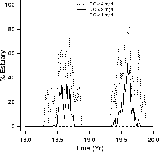
   FIG. B3. Percent of the entire estuary with a DO (mg/L) concentration falling within the given intervals over years 18 and 19.

 

   FIG. B4. Fig (a): Clam density over time (#/m$^2$). Fig (b): Clam biomass density over time (g/m$^2$). Fig (c): Background prey density (g/m$^2$) over time. All three variables appear to have stabilized after 20 years. Horizontal lines represent the average computed after year 10.

 

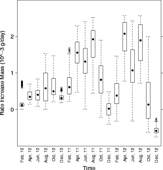
   FIG. B5. Rate of growth (g wet/day) of clams spawned in the spring and fall of year 10 over the subsequent 2.5 years. Clams are followed on 40 randomly selected fine-level triangles. The rate of growth slows considerably during the clam's first winter and they may loose mass during their second winter. The large variability in growth rates during summer results from the different depths temperatures and DO of the triangles.

 

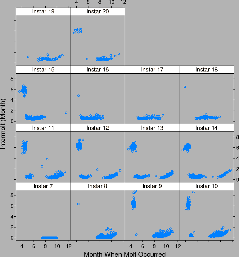
   FIG. B6. Length of time between successive molts by the month when the subsequent molt occurs and the instar of the molting crab. E.g., Instar 8 represents the time to go from instars 7 to 8.

 

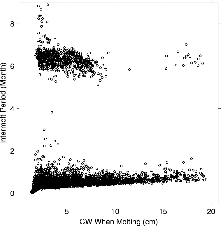
   FIG. B7. Length of time between successive molts by the CW of the molting crab.

 

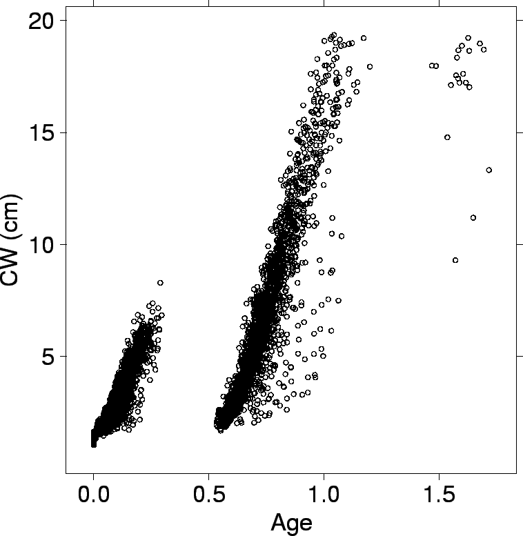
   FIG. B8. Crab age on CW.

 

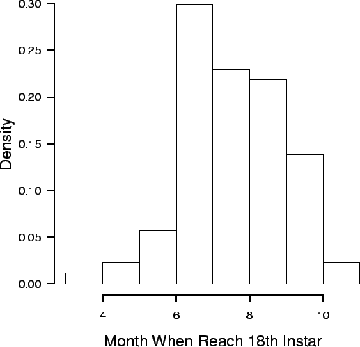
   FIG. B9. Distribution of month (April to October) when crabs reached the 18th instar.

 

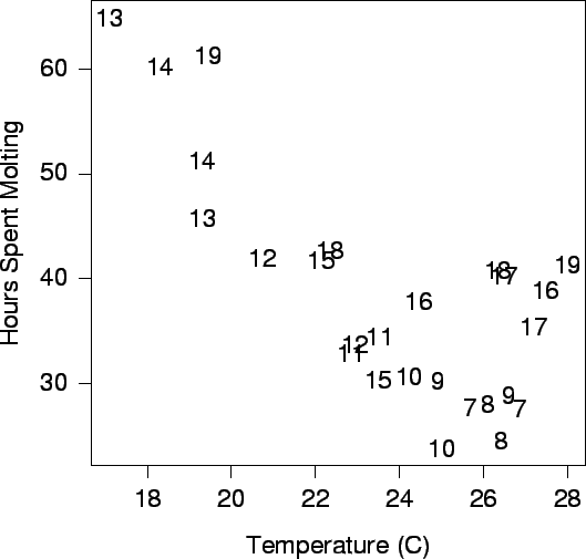
   FIG. B10. Amount of time two crabs took to molt at different instars (the numbers shown on the plot) and temperatures. The plot is based on the detailed life histories of two randomly selected crabs.

 

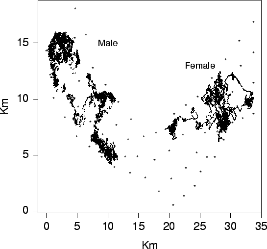
   FIG. B11. Paths of a male and female crab in the estuary over their lifetime.

 

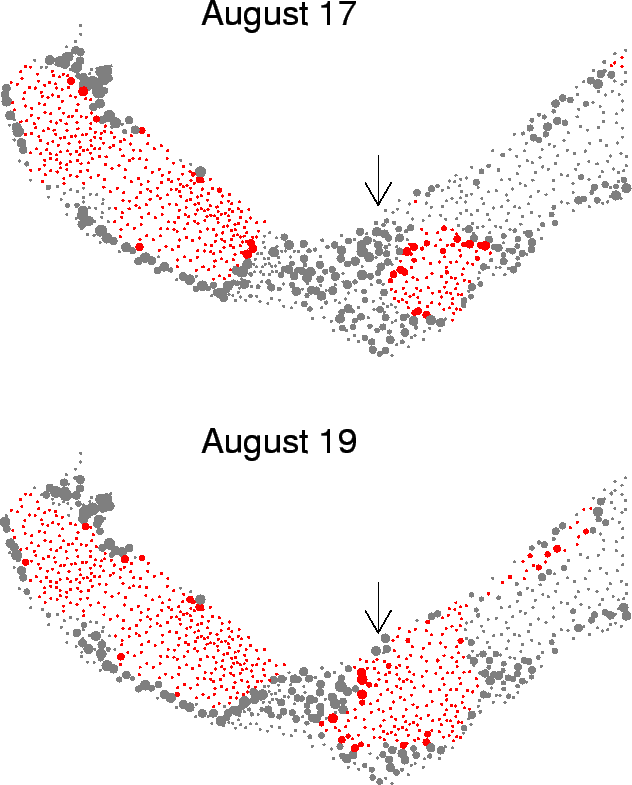
   FIG. B12. Each point represents a single fine-level triangle in the estuary. The size of the point represents the amount of crab biomass (g/m$^2$) on that triangle. The larger the point, the more biomass present. Red points indicate locations in the estuary experiencing a DO $<$ 3 mg/L. Gray points indicate DO $\geq$ 3. The arrows highlight the changes that occurred in crab biomass as a result of changing DO over August 17 to 19.

 

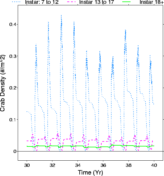
   FIG. B13. Time series of density (#/m$^2$) for 7-12, 13-17 and 18+ instar classes of crabs during years 30 to 39 over the entire estuary.

 

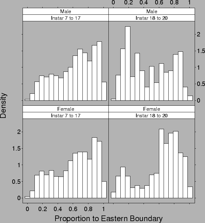
   FIG. B14. Density of crabs vs proportional distance to the eastern boundary of the estuary conditional on the sex and instar of the crab.

 

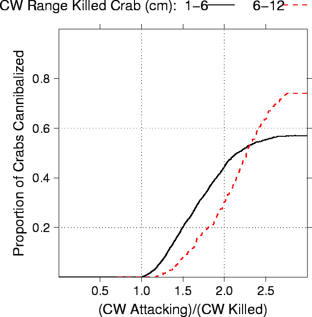
   FIG. B15. Proportion of two different size classes of crabs killed (CW 1-6 cm, and 6-12 cm) relative to the ratio of how much larger the attacking crab was. A smaller proportion of 1-6 cm CW crabs were cannibalized than 6-12 instar crabs - the other major cause of mortality for these small juvenile crabs being starvation. Second, the crabs killing the 1-6 cm CW crabs were on average a factor of $\approx 1.7$ larger while for 6-12 cm CW crabs the attacking crabs were on average larger by a factor of at least 2. In neither case was a large proportion cannibalized by similar sized conspecifics.

 

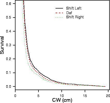
   FIG. B16. Effect on crab survival of altering the ratio of crab sizes at which death due to aggression is most likely (see Appendix B.4.6). Left, Def and Right correspond to $\mu = 1.5 , 2.0, 2.5$.