Ecological Archives E093-103-A1

David A. W. Miller. 2012. General methods for sensitivity analysis of equilibrium dynamics in patch occupancy models. Ecology 93:1204–1213.

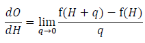
What are sensitivities? Sensitivity analysis is a general term used to specify an analysis that asks how changes in model components affect predicted outputs of the model. A "sensitivity" can be defined as a measure of how changes in a specific variable in a model affects values for a specific output. For example, we may want to know how sensitive the proportion of sites occupied by golden eagles, which we could denote with the variable O, is to changes in the abundance of hares, denoted by H. This can be expressed as a derivative and for the purposes of this paper I only use a strict definition of sensitivity as the first derivative of an output variable of interest with respect to changes in an input variable of interest. So in the eagle example, the sensitivity would be the derivative of occupancy with respect to hare abundance:

How should we interpret this? A sensitivity is a measure of absolute rate of change and has units defined by the units of O and H. It is the change in the proportion of occupied sites per unit change in hare abundance, or how quickly (and in which direction) does occupancy change as hare abundance increases. As with all derivatives, this rate depends on the values of the function that relates H to O. Thus, if we have two different systems and develop a model that describes how H relates to O for each, the functions that describe these relationships will likely differ and if they do the sensitivity will also likely differ. It is also important to note that the sensitivity is the rate of change at the exact value of H. If the relationship between O and H is non-linear then how closely the sensitivity predicts the response of O to changes in H will decrease as the amount H is perturbed increases. Thus, sensitivities are most accurate for predicting the effect of small changes in parameters. When very large changes are of interest, other perturbation analyses will be more appropriate. However, understanding what happen when we make small changes to the parameters in the model can provide important insights and is a good starting point when making inferences about a model.

How does this work in practice? Let's stick with the example of the sensitivity of eagle occupancy to changes in hare abundance. Say that we estimate parameters for our model to describes the relationship of H to O, and what we come up with is a simple linear model with an intercept and a slope where:

Making predictions in this case is straight-forward and we really don't need a formal sensitivity analysis to do what we already can already do informally. However, for purposes of illustration, this example is useful because we can match the intuitions we already have about how a regression model works, to the results we get when we calculate the sensitivity to a parameter in the model. As we defined sensitivity, it is the derivative of O with respect to H, and we get the value ? for the sensitivity of occupancy to changes in hare abundance (d/O/dH = β). That is, if we increase H, O will increase at a rate equal to β. This of course is how we already interpret a slope coefficient in a regression model and one definition of a derivative is that it is the slope (or tangent) of a function at a given value. In the case of a simple linear model, the derivative does not change as H changes, so the sensitivity is the same regardless of the current value of H.

Sensitivities are much more useful for understanding non-linear relationships and we can extend the current example to illustrate this. Let's now assume our model for the relationship between O and H is quadratic so that:

The sensitivity of occupancy to changes in hare abundance is (β + 2δH). We see that predicting the rate of change O is more complex in this case and also that the sensitivity depends on the current value of H. If δ is positive, then the rate at which occupancy increases, will increase as the current value of hare abundance increases. That is, the more hares there are, the greater the effect of increasing hare abundance further.

These examples ignore that O is a proportion and will need to be constrained to be between 0 and 1. Of course a good model should probably enforce this constraint. More important for our purposes, we are dealing with models that take a completely different form, where the relationship between O and H is more complex. Regardless, we can apply the same basic approach (estimating sensitivity based on derivatives), and the make the same interpretations (a description of the effect of changing a parameter). Dynamic occupancy models specify that O is a function of some set of transition parameters (e.g., extinction and colonization) and these in turn can be affected by underlying parameters such as hare abundance. Calculating sensitivities in this case is more challenging, but this additional complexity motivates the need for methods that can be used to understand how underlying parameters affect our predictions about state dynamics.

Frequently our goal will be to understand how temporal dynamics affect the probability a site is in a given state. At each time step, a site is in a discrete state that comes from a finite set of possible states. In the simplest models there are two possible states, which describe the occupancy status for a single-species, occupied and not occupied. The state distribution is a probability distribution that tells us the probability a given site is in each of the possible states.

We are not constrained to having only 2 states and many useful occupancy models use more than 2. These multistate models describe other characteristics of a site in addition to whether or not the focal species is present. Examples include the occurrence of a second species (MacKenzie et al. 2004; 2006), the relative abundance of individuals in an occupied site (Royle 2004; MacKenzie et al. 2009), whether breeding was successful in sites that are occupied (MacKenzie et al. 2009; Martin et al. 2009a), and the habitat state of a site (MacKenzie et al. 2011). In each case, an individual state is defined by a unique combination of the state characteristics, and all possible combinations need to be included. I considered a multistate occupancy model where occurrence of arroyo toads, occurrence of predators, and whether habitat is suitable are all measured at each time step. Because toads and predators can only occupy a site when the habitat is suitable, 5 possible states occur:

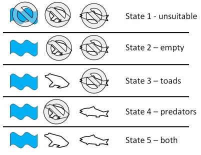
The state distribution in this case is the probability a site is in each of the 5 states. The 5 states are exhaustive (a site must be in 1 of these states) and therefore the probability of being in each must sum to 1.

A Markov process is one in which the state of a system only depends on the state in the previous time step. Thus no information is carried forward, the future state of a system only depends on the current state. Thus, it is independent of what has happened previously. How does this work in the case of an occupancy model? In our simplest model in which a site is either occupied or not occupied, the probability that a site will be occupied in the future only can depends on whether it is currently occupied. Therefore, a site that has been occupied for 5 years is no more likely to be occupied in the future, than one that has only been unoccupied for 4 years and only occupied for the last year. It is possible to build "memory" into models and still have a Markov process, but this involves defining additional states. For example, we may include a state which only includes sites that are currently occupied but were not occupied in the previous year and a separate state for sites that are currently occupied and were also occupied in the previous year. Green et al. (2011) provide an example of this type of Markov model in an occupancy context.

The type of Markov process model used for most occupancy models, and in all calculations I derived, is a discrete-time, finite-state Markov chain. They are discrete time because we model transitions that are measured at discrete time steps rather than those that occur continuously. In the multi-season occupancy model described by MacKenzie et al. (2003) a single measurable transition occurs from one season to the next. If in the interim between seasons an occupied becomes unoccupied and then is recolonized again, the sites is treated as having gone from the occupied state to the occupied state (i.e., all that is modeled is changes in states between the discrete times). Our models are finite-state in that the state of a site is one of a finite set of possible states (occupied or not occupied in our simplest models). The probability of being in each of these states must sum to 1 and generally we are going to be dealing with a smallish number of states. This will probably 2 to 5 states in most cases, although many more are possible and likely to be useful in certain applications. Finally, our model is a Markov chain because our Markov process occurs repeatedly over multiple time steps. In fact, what we hope to characterize is something about how the system functions as the Markov process is repeated over an extended set of time.

For a simple two-state occupancy model where sites are either occupied or not occupied by a species of toad, we get a model that works as follows.

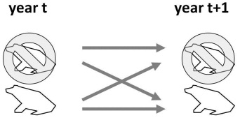
A site belongs to one of the 2 finite states (occupied or not) and states are measured at discrete intervals on an annual basis. This is a Markov process because the state in year t + 1 is solely a function of the state in year t. These transitions occur year after year creating a Markov chain which we can use to make predictions about the equilibrium system state.

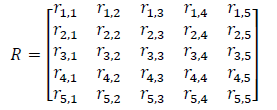
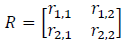
Consider a system like the toad model with 5 possible states. If a site is in the first state, there are five possible outcomes for the site in the next time step. It can remain in the first state, or it may transition to one of the other 4 states. The probability of each of these potential transitions occurring is called a state transition probability. The probabilities for each of the 5 possible transitions must sum to 1. A similar set of probabilities can be defined for sites that start in the second, third, fourth, and fifth states for a total of 25 combinations of starting and ending states (5 × 5). I denote the transition probability from state j to state i as r_I,j.

It is useful for calculations to organize the full set of transition probabilities in matrix format. If there are k possible states, our matrix R will be square with k rows and k columns. The transition probabilities should be assigned with each column representing a starting state and each row the ending state, so that:

An important property of the transition matrix is that it is column stochastic, that is, each column sums to 1. Once the transition probabilities are in matrix form, we can use matrix multiplication to ask, given a state distribution in time t what will the state distribution be in time t + 1. Use s(t) to denote a vector defining the state distribution in time t. Then:

where the multiplication of the matrix R and vector s is done using matrix multiplication.

For our purposes here, environmental variation is any case where the Markov transition matrix varies, either among sites or among time periods. These correspond to the two types of variation I considered, spatial and temporal. In many cases, using simpler models that do not include environmental variation may be sufficient, even when we know that a lack of variation will never be the case. However, if environmental variation is included, an alternative set of methods must be used to take this variation into account. Note that in the case of temporal variation, for all calculations I assume the mean transition probability is being perturbed. Thus, sensitivities measure effects of changes to the mean transition probability where the probability is increased a little bit for all years. Variance remains the same and I do not consider effects of changing the amount of variation.

A key concept for Markov chain models is the idea of the stationary state distribution. The stationary state distribution will have a slightly different interpretation depending on whether or not environmental variation occurs and I will start by defining it in the case with no variation.

We can illustrate the concept in a couple of ways. First, imagine a very large number of sites where the state distribution is the proportion of sites in each state. If transition probabilities are constant across time, in all but some limited cases, no matter what the starting distribution was, the state distribution will always converge to the same state distribution, which is referred to as the stationary state distribution. Generally this convergence is pretty fast, so it is a good measure of where things will end up given a particular set of transition probabilities and asking how the distribution changes when transition probabilities change has meaningful interpretation.

An alternative way to think about the stationary state distribution is to focus on a single site. In each time step the site is in one of the possible states and it transitions among states based on the transition probability matrix. If we record the state of the site over a very large number of transitions, the stationary state distribution will be the proportion of time steps the site is in each of the states. Thus, the stationary state distribution is the probability at any time step a site will be in each of the states. This definition is useful because we can draw an equivalent understanding when dealing with temporal variation.

One way to calculate the stationary state distribution is to start with a value for s and multiply it by R a very large number of times until we are satisfied we have converged on a value. A much easier and useful way to calculate the distribution is to use a standard eigenanalysis. This can be done with most standard computing programs and the eigenvector associated with the dominant eigenvalue of R is used. Once calculated all we have to do is rescale the eigenvector to sum to 1. If you are not familiar with eigenanalysis, do not worry. I provide the code for the calculations in the supplements and Caswell (2001) is a great resource if you want to learn more.

Our intuitions have to shift slightly if we include environmental variation. In the case of spatial variation, the stationary state distribution is still the proportion of all sites in each state once convergence is reached (think of it as the weighted mean of a more than 1 population of sites). Using our second definition, the stationary state distribution when spatial variation occurs is the mean probability any site is in a given state during any time step. As noted in the paper, calculating the stationary state distribution in this case involves calculating weighted means of the stationary state distribution for each possible set of state dynamics.

Our understanding needs to shift some when we consider temporal variation. An important assumption is that variation among time steps in transition probabilities is stationary. That is, the mean does not change across time and the probability of any set of transition values is the same across time. In this case, we can again imagine a large number of sites where the proportion of sites in each state is described by the state distribution. When we draw random sets of transition matrices, because they are variable, we will not converge to a single value but instead the state distribution will vary around some expected value. The stationary state distribution in this case can be thought of as the mean proportion of sites in each state across a long time period.

We can also consider our case where we track a single site across time. In this case our interpretation is exactly the same as when no temporal variation occurred. The stationary state distribution is the probability after enough time for convergence that at any time step the site is in a given state. In most cases if we removed temporal variation and just calculated the stationary state distribution from mean transition probabilities, the value will be very close to the stationary state distribution if we kept the temporal variation.

In cases where temporal variation occurs, I use simulation to calculate the stationary state distribution. A starting value is picked and the state distribution is projected across many thousands of time steps. The mean distribution is then calculated for the sequence.

When we make inferences from the stationary state distribution they are based on how changing parameters will influence equilibrium dynamics. We do this by examining how changes affect the stationary distribution, which is a long-term average at equilibrium. This may be a poor measure of outcomes in cases where: non-stationary occurs, that is transition rates among states are changing systematically across time; or if we are interested in transient dynamics, such as when the current state distribution is far from the stationary state distribution and interest is in what occurs in the short-term (before the population approaches equilibrium). Sensitivities based on the equilibrium distribution will be of primary interest for understanding system dynamics in most cases and are a good starting point for understanding model dynamics.

As stated previously, the probability of occurring in each of the system states must sum to 1. Similarly the probability a site that was in a given state is in each of the possible states in the next time step must also sum to 1 (columns of the transition matrix). This is sensible because although the state of the site can change through time it must always belong to one of the possible states. This constraint is important to consider when calculating sensitivities. Say that we have 5 possible states and we want to determine how increasing transitions from the 3rd to 5th state affects the stationary distribution. We must take into account that increasing this transition is only possible if transitions to the other 4 states (3rd to 1st, 2nd, 3rd, or 4th) decrease by an equal amount. If this "compensation" does not occur, the probabilities would sum to a value greater than 1. When calculating sensitivities this constraint should always be maintained and I refer to this as the Markov constraint since it is derives from the properties of Markov transition matrices. The same constraint is not necessary for sensitivity analyses of non-Markov matrices such as commonly used in population models. Luckily in most cases, the way that we construct occupancy models to include lower-level parameters will almost always mean this constraint is met without extra work. In cases where this is not the case, such as when we calculate the sensitivity of the stationary state distribution (e), to changes in transition probabilities (r_i,j), a compensation method will need to be used to maintain the constraint.

The approach I take for calculating sensitivities is to break an occupancy model into a set of component functions, calculate derivatives for each, and then combine them using the chain-rule (see Part II for a more detailed description of the approach). In all calculations, one of the components will be the sensitivity of the stationary state distribution to changes in the values of the transition matrix. It is useful to distinguish other functions that make up the model by how they relate to this central component.

First, consider what I have referred to as lower-level parameters. These are parameters used to calculate the transition probabilities of the transition matrix. The transition probability may be a function of other nested transition probabilities (i.e., conditional binomial formulations) or of some covariate that predicts is used to predict the transition value. A lower-level parameter is parameter that occurs in a function which predicts at least one transition probability.

The other type is what I have referred to as derived state variables. These are variables which can be calculated as a function of the stationary state distribution. This can include the ratio of the probability of being in 2 states, the probability of being in more than one state, or some more complicated function such as a diversity measure. In each case, the derived variable will be a function of the proportions that make up the stationary state distribution.

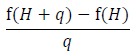
Whenever possible it is best to directly calculate the derivatives that make up the sensitivity calculations we are interested in. However, in some cases this will not be possible and in others an alternative method for calculating values is a useful approach for checking calculations. One method to approximate the actual derivate is to calculate sensitivities by numerical perturbation. The idea behind this approach can be illustrated by looking at one definition of a derivative. Using our previous example, the sensitivity of occupancy to hare abundance is the derivative of O with respect to H. As stated previously, the derivative measures the rate of change, ΔO/ΔH, at the current value of H. We can derive this value by first asking how O changes given a small change q in H, which is expressed as:

where O = f(H). The derivative is then defined as the limit of this equation as q approaches 0:

As q gets smaller and smaller and closer and closer to 0 the value for the Eq. A1 converges to the actual derivative. Numerical perturbation takes advantage of this by choosing a value of q that is close to 0 and using Eq. A1 as an approximation of the derivative. We want this value to be as small possible, but in practice we will be using a computer to calculate the value and we are constrained by the precision of the program we are using. If q is too small, say 10^-100, we are not going to have the precision to measure the change in O. In practice therefore, we need to pick a small value, but not too small. I have generally used a value around 10^-4 for q and have found differences between estimates using this method and the true derivative are the same out to at least 4 or 5 significant digits in the applications I have attempted.

Numerical perturbations are principle method used for all calculations I derive which include temporal variation. I also find this approach useful as a check for other sensitivity calculations to make sure I have set the equations up correctly the first time I try to calculate them.

For a more complete description of sensitivity analysis, types of sensitivity calculations, and there use in ecological models one should consult Caswell (2001). Although most of his text is focused on population models rather than Markov-chain models, the same basic principles apply. The book also has a short treatment of eigenvector sensitivities (section 9.4) and its application to analyses of Markov-chains (section 9.6). Other important ecological references with applicability to occupancy models are Hill et al. (2004), Caswell (2007, 2009), Martin et al. (2009b), and Green et al. (2011).

My goal was to set up a framework which can easily be modified when calculating sensitivities which involve the stationary state distribution of Markov chain models. The types of sensitivities calculations found in the paper are by no means an exhaustive treatment of potentially interesting relationships. However, the same basic approach can be extended to tackle many additional relationships. I'll illustrate how I have done this with some examples. To make it easier I will deal first with cases where there is no environmental variation and then demonstrate how to calculate similar values when temporal and spatial variation occurs. I concentrate on calculation of 2 example sensitivities, which differ in complexity:

Example 1: The example uses a common model in metapopulation literature that includes the potential for rescue effects in the formulation. For this model, I show how to calculate the sensitivity of occupancy to changes in colonization.

Example 2: The second example is for the arroyo toad model that was used as the first example in the paper. I extend the model presented there to also include an effect of water depth (D) on toad extinction where the relationship uses a logit-link to relate the two. In this example I calculate the sensitivity of co-occurrence to changes in water depth.

The basic steps for calculating sensitivities when no environmental variation occurs are:

(1) Divide the relationship into constituent functions. Most importantly we want to separate the relationship between the transition matrix and the stationary state distribution from those that involve lower-level parameters and derived state variables. In some cases, it will also be useful to divide lower-level parameters and derived state variables into additional pieces. All of the sensitivities considered in the paper include the sensitivity of the stationary state distribution to changes in transition parameters as a component. Being able to treat this as a separate derivative is the key to efficient calculations.

(2) Calculate derivatives for each of the functions. Once separated, calculating derivatives for lower-level parameters and derived state variables will generally be straight forward. Calculating the derivatives involving the stationary state distribution with respect to elements of the transition matrix demands some advanced calculus. Luckily an efficient equation for this has been derived by others (Caswell 2001; Hill et al. 2004) and it is easy to implement.

(3) Combine the parts using the chain-rule to calculate the sensitivity for the complete relationship. Once we have derivatives for each of the functions, we recombine them using the chain rule. In reassembling the parts we will need to account for all the possible pathways by which the input variable of interest can affect the output variable of interest.

Example 1: The first example is relatively simple, in that we only have to divide the sensitivity into 2 constituent functions. As I noted in the paper, the transition matrix in Eq. 16 can be modified to account for rescue-effects can be constructed where the new transition matrix is specified as:

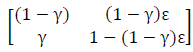
The transitions are a function of 2 parameters, γ for colonization and ε for extinction. The rescue-effect results because when extinction occurs the model allows for the possibility that the site may be recolonized in the same time step.

There are two possible states for a site, unoccupied and occupied, and the stationary state distribution is the equilibrium probability a site is in each of these states. The second value in the vector, e₂, is the equilibrium probability of being occupied. Our goal is to calculate the sensitivity of occupancy (e₂) to changes in the colonization probability (γ). Expressed as a derivative, the sensitivity we are interested in is:

Note that the Markovian constraint is naturally met in this case. If we change γ, the columns of the transition matrix above still sum to 1 (e.g., in column 1 if γ increases, [1 - γ] decreases by an equal amount).

Step 1: divide this relationship into its constituent parts. In this case we can divide the relationship into two functions: the effect of the transition parameters (r_i,j) on the stationary state distribution (e), and the effect of colonization on the transition parameters.

In the first part, we have a transition matrix, which we use to calculate the equilibrium occupancy estimate e₂,

We divide this from the functions involving lower-level parameters which describe how each of these elements are themselves a function of γ and ε:

r_1,1 = 1 - γ

r_2,1 = γ

r_1,2 = (1 - γ)ε

r_2,2 = 1 - (1 - γ)ε

Step 2: take the derivative of the component functions. We need to calculate the derivatives of occupancy with respect to the transition parameters, ∂e₂/∂r_i,j, and the derivatives of the transition parameters with respect to colonization, ∂r_i,j/∂γ. The first are calculated using Eq. 6 in the text. The second component is made of conditional binomials and can be treated similarly to the example in the paper.

∂r_1,1/∂γ = -1

∂r_2,1/∂γ = 1

∂r_1,2/∂γ = -ε

∂r_2,2/∂γ = ε

Step 3: combine the individual components using the chain rule. In this case where we only have a lower-level parameter we can use Eq. 9. Our goal is to sum up all the potential paths by which colonization can affect occupancy through our different components of the model. In this case colonization can affect each transition probability individually, and each of these transition probabilities can affect occupancy so we must sum all 4 pathways. What we end up is this equation:

de₂/dγ = -1 × ∂ e₂/∂r_1,1 + 1 × ∂e₂/∂r_i,j - ε × ∂e₂/∂r_i,j + ε × ∂e₂/∂r_i,j

Example 2: The second example is more complicated in that we have 5 possible states and the sensitivity includes both lower-level parameters and derived-state variables.

Step 1: divide into constituent functions. In this case we will separate out the functions which determine the derived state variables and which include the lower-level parameters. We also will want to divide the lower-level component even further to make the calculations easier. The component parts are:

(1) The effect of water depth on toad extinctions. Remember toad extinction depends on whether a site was unoccupied or occupied by predators in the last time step so we have two functions to deal with. Let's say the functions look like this:

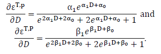
logit(ε^T,p) = α₀ + α₁ × D
logit(ε^T,P) = β₀ + β₁ × D

(2) The effect of toad extinction on the transition probabilities. The relationship between each of the transition parameters and the underlying conditional binomial parameters (including extinction) are found in Table 1 in the main text.

(3) The effect of transition probabilities on the stationary state distribution. Just like the other example the equilibrium state vector e is a function of the elements of the 5 × 5 transition matrix R

(4) The relationship of the stationary state distribution to co-occurrence. Using C to denote co-occurrence, it is calculated as:

C = e₅/(e₃ + e₅)

Step 2: Now we need to calculate derivatives for each part.

(1) For logit-link functions, Eq. 14 can be used. The derivatives are:

(2) We need to calculate ∂r_i,j/∂ε^T,p and ∂r_i,j/∂ε^T,P for each of the possible combinations (see Table 1 again for the functions for which the derivatives are calculated). Although there are 25 total transition probabilities, the derivative will be 0 for all transitions that do not include the extinction parameter so this narrows it down to 4 non-zero transition probabilities for each.

∂r_2,3/∂ε^T,p = (1 - ε^H) × (1 - γ^P,T)

∂r_3,3/∂ε^T,p = -(1 - ε^H) × (1 - γ^P,T)

∂r_4,3/∂ε^T,p = (1 - ε^H) × γ^P,T

∂r_5,3/∂ε^T,p = -(1 - ε^H) × γ^P,T

and

∂r_2,3/∂ε^T,P = (1 - ε^H) × ε^P,T

∂r_3,3/∂ε^T,P = -(1 - ε^H) × ε^P,T

∂r_4,3/∂ε^T,P = (1 - ε^H) × (1 - ε^P,T)

∂r_5,3/∂ε^T,P = -(1 - ε^H) × (1 - ε^P,T)

(3) The derivatives, ∂e/∂r_i,j, are calculated using Eq. 6.

(4) For the derivative of a ratio, Eq. 22 can be used as an example.

∂C/∂e₃ = -e₅/(e₃ + e₅)²
∂C/∂e₅ = -e₅/(e₂ + e₅)²

Step 3: bring everything back together. The basic idea here, as illustrated by Eq. 9–11, is to sum across all the levels of each of the components. So we have 2 extinction parameters affected by water-depth, i times j transition parameters that can be affected by lower-level parameters, and 5 elements of the stationary state distribution that can be affected by transitions. Putting all them together we get an expression that looks like this:

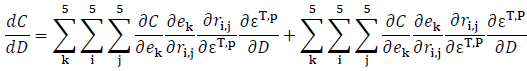
The equation sums across the two extinction parameters, the 5 rows and 5 columns of the transition matrix and the 5 elements of the state vector.

When dealing with a population of sites, where not all sites have the same dynamics it is possible to incorporate this spatial variation in to sensitivity estimates. Sites, or groups of sites, can be classified according to a set of unique model parameters associated with the site. Sensitivities can either relate to changes in parameters within sites or changes in the proportion of sites in each of the possible classes.

In the first case we are perturbing a parameter in the dynamic model for the site, but because sites differ in their dynamics, the effect will differ among sites. We can capture that variation by calculating the average effect of the change across all sites or a weighted average across classes. So in example 1, say we have 100 sites in our population, each of which have a different inherent probability of colonization and extinction. We can calculate the sensitivity of occupancy to changes in colonization for each of the 100 sites and the simple average of these sensitivities will tell us how sensitive mean occurrence for the population of sites is to a similar change in the colonization probability of all sites. For the arroyo toad model, as noted in the paper, 43.3% of sites in the system were classified as perennial streams, with the remaining classified as ephemeral. If we could change water depth in all sites simultaneously we could ask what the sensitivity of co-occurrence for the system as a whole is to changes in water depth. To do this we would calculate the sensitivity in each system and then calculate the weighted average to get a global sensitivity.

The second case of spatial variation relates to times when changes do not occur to the dynamics within a class per se. Instead the proportion of sites in each class could change. A good example of this is if we were to ask how sensitive the stationary state distribution in the arroyo toad model is to changes in the proportion of perennial sites. This calculation is made using Eq. 27. We can then consider lower-level parameters which may affect the proportion of sites which are perennial or derived state variables such as co-occurrence. Again the chain-rule would apply and the derivatives of the component functions can be used to calculate the sensitivity for the whole.

The solution I propose when temporal variation is less elegant than other calculations because there is not a closed form solution. Instead, simulation and numerical perturbation can be used to approximate derivatives (see definitions in Part I for a detailed description of how numerical perturbation works). As a result, the approach used for setting up calculations will differ significantly from the one used for models without temporal variation. The steps to calculate the sensitivity of the stationary state distribution to changes in an input parameter are:

(1) Develop a set of potential transition matrices. In many cases the parameters for our occupancy model are estimated and include estimates for each time step in the data set (e.g., transition matrices for the arroyo toad model were estimated for 7 unique years). One can use this finite set of estimated matrices as our set of potential matrices, assuming each has an equal probability of occurring in a given time step. Alternatively one could define the potential transition of matrices to come from a continuous distribution, where there are an infinite number of possibilities each of which occur at a probability defined by the probability density function.

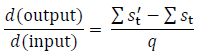
(2) For each matrix R in the potential set, define a second perturbed matrix R'. The approach used in numerical perturbation is to change our input variable by a small amount q and look at how it affects our output variable of interest. Thus R' is calculated by increasing the input variable of interest by a small value q.

(3) Project a long series of randomly chosen transition matrices from both the original and perturbed set. I consider temporal variation where the transition matrix is chosen independently of the transition matrix in the last time step (i.i.d. matrix selection). This process is simulated by randomly choosing, with replacement, a sequence of matrices from the potential matrix set. For each matrix, select the corresponding R' matrix, maintaining the same order with the perturbation being the only difference between the sequences. Next project these matrices, starting with an initial state distribution (s₀) and multiplying this by the transition matrices in order (Eq. 3), recording the state distribution at each time step (s_t for the original sequence and s_t' for the perturbed sequence). Maintaining the same sequence and using the same starting values will maximize the efficiency of the calculation

(4) Use the simulated state distributions to calculate the sensitivity. We will now have two long sequences of state distributions, one for the original transition matrices and one for the perturbed matrices. We can now use Eq. A1 to approximate the sensitivity:

It is best to throw out the initial calculated state distributions to avoid transient dynamics (say the first 100 iterations). And, the more iterations that are simulated, the better the estimate will be.

Example: Let's illustrate this using the arroyo toad model and calculating a sensitivity of mean co-occurrence probability among years to changes in the mean water depth among years. Note now that our stationary state distribution represents the mean probabilities of being in each of the age classes across many years and what we are perturbing is the mean value of water-depth, which may vary among years since we are allowing for temporal variation.

Step 1: identify the set of potential matrices. In our example there were 7 years for which transitions were estimated and we could use these as our set of matrices to capture the observed variation seen during the period of the study. For each year we need to calculate a transition probability matrix R based on the parameters for the model in that year.

Step 2: develop a set of perturbed matrices. We need to recalculate our transition probabilities again. However, this time we will increase water depth (D) in each of the years by a small value q (say 0.0001) and calculate R'. This new set represents transitions when the mean value of D is increased (but the variance remains the same).

Step 3: project matrices. We will draw matrices randomly maintaining the same order for the original and perturbed matrices. Then for each we project the system forward through time recording the state at each time step. To do this we pick a starting value s₀ and multiply it by the first matrix. We record the resulting value s₁ and then multiply that by the second matrix. Ideally we will want to continue this for a large number of iterations, say 10,000.

Step 4: We use the resulting values for the state distribution to calculate our sensitivity. First we will throw out the first 100 iterations because the system may have been in a transient state. Then we take the remaining values (101 to 10000) and average these for both the original and perturbed sequence. These average values are our estimates of the stationary state distribution when temporal variation occurs (e[T]). Using our rules for numerical perturbation we subtract the 2 values and divide them by the amount of the perturbation q to get an estimate of the sensitivity/derivative.

When both types of environmental variation are considered, the temporal component will be dealt with first and then the spatial component can be incorporated. For example in our water depth example if we wanted to incorporate differences for perennial and ephemeral streams we would first calculate the temporal sensitivity for each system and then calculate the weighted average to get a system wide sensitivity.

Putting this into practice in an efficient way will involve implementing the calculations in a computing package. I have chosen to use R because it is free, widely used, and will be familiar to many. Using scripts and functions will allow calculations to be repeated with different model parameters and for the sensitivities for multiple input parameters to be calculated simultaneously. I have provided a set of useful functions that can be called to calculate derivatives that will commonly be used in applications (Supplement 1) and provide code for all of the sensitivities that are shown for the 3 example models. Here I provide further background on how to use the code. I begin by showing how to calculate derivatives for a variety of component functions for sensitivity relationships (step 2 in our algorithm) and then give examples of how these can be combined using the chain rule (step 3). All snippets of code come from the examples in the supplements.

All of the functions in Supplement 1 should be loaded. Therefore, running the script in Supplement 1 is necessary before working with the following examples. The arroyo toad data sets should already be loaded to run the examples. The code to do this is:

There are two matrices which do not include environmental variation: perD for perennial streams and ephD for ephemeral streams. The set of annual matrices used when temporal variation is included at perT and ephT for perennial and ephemeral streams, respectively.

The stationary state distribution is a useful starting point for analyses. For the case where no temporal variation occurs we get e with the function sens.

If we wish to include spatial variation and get an estimate of the stationary state distribution for the system as a whole e(S), we calculate the weighted average of the 2 stream types.

And finally if we wish to include both temporal and spatial variation to get e(T,S) we will calculate the weighted average of the temporal estimates.

Derivative of stationary state distribution with respect to transition probabilities

This is the derivative that will occur in all calculations. The set of functions in Supplement 1 primarily deals with generating this value. Functions are provided to calculate values with and without a method for compensation. Uniform or proportional compensation will generally be used when interest is only in the relationship of transition probabilities to the state distribution or a derived state variable. In most cases, the formulation of the lower-level parameters will maintain the Markovian constraint and the partial derivatives will be combined via chain-rule with other derivatives.

For no environmental variation the partial derivatives (Eq. 5 and 6) are calculated using the function sens.

This returns an i by j by k matrix where the indices correspond to ∂ek/∂r_i,j. To calculate sensitivities with uniform and proportional compensation, use the function markov.sens.

dedR.ephD.uniform <- markov.sens(ephD)$unif
0 dedR.ephD.proportional <- markov.sens(ephD)$prop

To generate the same sensitivities with compensation when temporal variation occurs, use the functions unif.Tsens and prop.Tsens.

dedR.ephT.uniform <- unif.Tsens(ephT)$sens
dedR.ephT.proportional <- prop.Tsens(ephT)$sens

I do not include an equivalent function to sens for the partial derivatives because the steps for calculating sensitivities with temporal variation when lower level parameters are included do not involve breaking the function into parts.

Derivatives of conditional binomial functions are generally pretty simple to calculate. What we want to do is calculate the derivative of each of the transition probabilities to the conditional binomial parameters and frequently there will be multiple conditional binomial parameters we are interested in. This can involve a lot of separate functions and automating this will speed the process. Here is how I set this up for the arroyo toad example, which included 25 transition probabilities and 12 parameters to define the probabilities.

dR.dTheta <- array(0,c(5,5,12))

cb <- c("gH","eH","gTu","gTp","gTP","eTp","eTP","gPu","gPt","gPT","ePt","ePT")

dR.dTheta[1,1,] <- attr(eval(deriv(~(1-gH),cb)),"gradient")
dR.dTheta[2,1,] <- attr(eval(deriv(~gH*(1-gTu)*(1-gPu),cb)),"gradient")
dR.dTheta[3,1,] <- attr(eval(deriv(~gH*gTu*(1-gPu),cb)),"gradient")
dR.dTheta[4,1,] <- attr(eval(deriv(~gH*(1-gTu)*gPu,cb)),"gradient")
dR.dTheta[5,1,] <- attr(eval(deriv(~gH*gTu*gPu,cb)),"gradient")

dR.dTheta[1,2,] <- attr(eval(deriv(~eH,cb)),"gradient")
dR.dTheta[2,2,] <- attr(eval(deriv(~(1-eH)*(1-gTp)*(1-gPt),cb)),"gradient")
dR.dTheta[3,2,] <- attr(eval(deriv(~(1-eH)*gTp*(1-gPt),cb)),"gradient")
dR.dTheta[4,2,] <- attr(eval(deriv(~(1-eH)*(1-gTp)*gPt,cb)),"gradient")
dR.dTheta[5,2,] <- attr(eval(deriv(~(1-eH)*gTp*gPt,cb)),"gradient")

dR.dTheta[1,3,] <- attr(eval(deriv(~eH,cb)),"gradient")
dR.dTheta[2,3,] <- attr(eval(deriv(~(1-eH)*eTp*(1-gPT),cb)),"gradient")
dR.dTheta[3,3,] <- attr(eval(deriv(~(1-eH)*(1-eTp)*(1-gPT),cb)),"gradient")
dR.dTheta[4,3,] <- attr(eval(deriv(~(1-eH)*eTp*gPT,cb)),"gradient")
dR.dTheta[5,3,] <- attr(eval(deriv(~(1-eH)*(1-eTp)*gPT,cb)),"gradient")

dR.dTheta[1,4,] <- attr(eval(deriv(~eH,cb)),"gradient")
dR.dTheta[2,4,] <- attr(eval(deriv(~(1-eH)*(1-gTP)*ePt,cb)),"gradient")
dR.dTheta[3,4,] <- attr(eval(deriv(~(1-eH)*gTP*ePt,cb)),"gradient")
dR.dTheta[4,4,] <- attr(eval(deriv(~(1-eH)*(1-gTP)*(1-ePt),cb)),"gradient")
dR.dTheta[5,4,] <- attr(eval(deriv(~(1-eH)*gTP*(1-ePt),cb)),"gradient")

dR.dTheta[1,5,] <- attr(eval(deriv(~eH,cb)),"gradient")
dR.dTheta[2,5,] <- attr(eval(deriv(~(1-eH)*eTP*ePT,cb)),"gradient")
dR.dTheta[3,5,] <- attr(eval(deriv(~(1-eH)*(1-eTP)*ePT,cb)),"gradient")
dR.dTheta[4,5,] <- attr(eval(deriv(~(1-eH)*eTP*(1-ePT),cb)),"gradient")
dR.dTheta[5,5,] <- attr(eval(deriv(~(1-eH)*(1-eTP)*(1-ePT),cb)),"gradient")

There are 25 functions that define the relationship between the transition probabilities and conditional binomial parameters (see Table 1). This code goes through each and calculates the derivative for each of the 12 lower-level parameters stored in the list cb. A similar example can be found in Supplement 1, which contains code for the golden eagle model.

In the golden eagle occupancy model (Appendix B; Supplement 1) I calculated the derivative of a conditional binomial parameter R with respect to changes in hare abundance (hare).

Ri = -0.775 ### intercept logit function for R
Rh = 5.948795 ### slope for hare effect logit function for R
dR.dHARE <- Rh*exp(Rh*hare+Ri))/((exp(2*Rh*hare+2*Ri))+(2*exp(Rh*hare+Ri))+1)

In the butterfly example, one component of the sensitivity of occupancy to patch area was the derivative of extinction to patch area (Eq. 17). For H. comma at the mean patch area the following code was used for this derivative:

We also need to calculate derivatives of derived state variables. A good example of this was calculating co-occurrence probability for predators when toads were present. This is a ratio involving to values from the stationary state distribution vector e₃ and e₅.

dCde3 <- -SSD.ephD[5]/((sum(SSD.ephD[c(3,5)]))^2)
dCde5 <- SSD.ephD[3]/((sum(SSD.ephD[c(3,5)]))^2)

Once the derivatives for the component functions are calculated the final step is to recombine them to get the overall sensitivity.

Example 1: Let's start with the sensitivity of the stationary state distribution to changes in the conditional binomial parameters of the arroyo toad model. Table 2 contains the full set of calculated sensitivities, which we will recreate. The output will be a matrix with 12 rows, one for each of the conditional binomial parameters, and 5 columns, one for each of the states in the stationary state distribution.

Begin with a single calculation, the derivative of e₁ with respect to changes in γ^H. We need to sum across all the transition probabilities (5 by 5).

We can extend this to get the sensitivities in Fig. 2a. The code calculates the deriviative of the derived state variable co-occurrence (C) with respect extinction and colonization parameters summed across all starting states. Two extensions are necessary, adding the relationship between the state distribution and co-occurrence, and combining extinctions and colonizations.

dedCB2.ephD <- rbind(dedCB.ephD[1:2,],colSums(dedCB.ephD[3:5,]), colSums(dedCB.ephD[6:7,]),colSums(dedCB.ephD[8:10,]),colSums(dedCB.ephD[11:12,])) #### this sums across all starting states for each of the extinction and colonization paramters

rownames(dedCB2.ephD) = c("gH","eH","gT","eT","gP","eP")

dcooccurdCB2.ephD <- dedCB2.ephD[,3]*-SSD.ephD[5]/((sum(SSD.ephD[c(3,5)]))^2) + dedCB2.ephD[,5]*SSD.ephD[3]/((sum(SSD.ephD[c(3,5)]))^2) #### combines the derived state variable - cooccurrence

Example 2: Now let's look at code for the butterfly metapopulation model. The goal here is to calculate the sensitivity of occupancy (e₂) to changes in area of the patch. The relationship is a function of a couple of estimated parameters in the function which predicts extinction probability and the colonization probability. For an average sized patch for the H. comma population with a colonization fixed to be 0.4 the following code calculates the sensitivity:

e = 0.010
x = 1.009
A = 0.94
E = e/(A^x) ## extinction, which is a function of e, x, and A
C = 0.4 ## colonization

R <- matrix(c((1-C),C,E,(1-E)),2,2) ## transition matrix (Eq. 16)
R.sens <- sens(R)$sensitivities
dR.dE <- matrix(c(0,0,1,-1),2,2)
dE.dA <- -e*x*(A^(-x-1))

de2.dA <- sum(dE.dA*dR.dE*R.sens[,,2])

The original function gets divided into 3 parts. The derivative of in occupancy with respect to transition probabilities (R.sens[,,2]), the derivative of the transition probabilities with respect to extinction (dR.dE), and the derivative of extinction with respect to changes in patch area (dE.dA). The first 5 lines of code define the parameter values for which the sensitivity is calculated. The next 4 set up and calculate the derivatives. Finally the last line of code uses the chain-rule to combine the parts (Eq. 18 in the paper).

Accounting for spatial variation is straight forward. For the arroyo toad model the sensitivity of co-occurrence for the overall population of sites in both stream types to each of the extinction and colonization parameters is the weighted averaged of the sensitivities. To do this we would use the following code:

The sensitivity of the stationary state distribution to changes in the proportion of ephemeral sites would be (Eq. 27):

The primary function I created to calculate these sensitivities is lower.Tsen (found in Supplement 1). The function uses numerical perturbation and simulation to calculate the sensitivity of the stationary state distribution e(T) to changes in a lower level parameter. In cases where the interest is in a derived parameter, it will output the mean simulated state distributions. The derived variable can be calculated for the original and perturbed matrices and Eq. A.1 can be used to then generate the sensitivity.

Let's step through how the function works, first calculating the sensitivity of the stationary state distribution to changes in each of the extinction and colonization parameters for the arroyo toad model. The first step in calculating this was to formulate our set of potential matrices R. We will use the estimated values for each of the years perT and ephT, which were generated at the beginning of this section. These are 3 dimensional arrays with the first two dimensions specifying the elements of the transition matrix and the third dimension relates to each of the years in the data set.

The second step is to calculate the perturbed matrices R', which correspond to each of the matrices R. This is done by adding a small value, q, to the lower level parameter of interest. I did not discuss it at the beginning of the section but I used a function called matrix.builder to build the transition matrices from the conditional binomial parameters. This was useful because it automated the process and I use the function again here, just changing input variables by a small amount. So the set of R' matrices when γ^H is perturbed can be calculated by:

An alternative set for each of the other extinction and colonization parameters is generated by:

mat.eH <- matrix.builder(tp + c(rep(0,6),rep(q,6),rep(0,12)))$matR
mat.gT <- matrix.builder(tp + c(rep(0,14),rep(q,3),rep(0,7)))$matR
mat.eT <- matrix.builder(tp + c(rep(0,17),rep(q,2),rep(0,5)))$matR
mat.gP <- matrix.builder(tp + c(rep(0,19),rep(q,3),rep(0,3)))$matR
mat.eP <- matrix.builder(tp + c(rep(0,22),rep(q,2)))$matR

When a derived state variable is not used, the function lower.Tsens will accomplish our 3rd and 4th steps of simulating and using them to approximate the derivative. The function has 3 input values that are necessary: the matrix set of R as a 3 dimensional array, a corresponding set of perturbed matrices R' in the same format, and the value that was used for q when generating R'. It also has a default of 10000 burnin iterations and 100000 total simulations and this can easily be modified if desired. The code for each of the extinction and colonization parameters is:

deT.dgH <- lower.Tsens(perT,mat.gH,q)$sens
deT.deH <- lower.Tsens(perT,mat.eH,q)$sens
deT.dgT <- lower.Tsens(perT,mat.gT,q)$sens
deT.deT <- lower.Tsens(perT,mat.eT,q)$sens
deT.dgP <- lower.Tsens(perT,mat.gP,q)$sens
deT.deP <- lower.Tsens(perT,mat.eP,q)$sens

The same approach can be used for any lower level parameter. All that matters is that R' be calculated by adding q to whatever lower level parameter is of interest.

Of course we still want to be able to deal with derived state variables. There are many possible derived parameters so building a single function to output all of them would not be possible. Instead we can use lower.Tsens to output the mean simulated state distributions, calculate the derived parameter for both the original and perturbed values, and use Eq. A.1 to calculate the sensitivity. Notice in the above code I followed the lower.Tsens function with $sens. To get the mean state distribution for the original matrices we use $e.T and for the perturbed matrices we use $p.T.

egH <- lower.Tsens(perT,mat.gH,q)$e.T
eeH <- lower.Tsens(perT,mat.eH,q)$e.T
egT <- lower.Tsens(perT,mat.gT,q)$e.T
eeT <- lower.Tsens(perT,mat.eT,q)$e.T
egP <- lower.Tsens(perT,mat.gP,q)$e.T
eeP <- lower.Tsens(perT,mat.eP,q)$e.T

pgH <- lower.Tsens(perT,mat.gH,q)$p.T
peH <- lower.Tsens(perT,mat.eH,q)$p.T
pgT <- lower.Tsens(perT,mat.gT,q)$p.T
peT <- lower.Tsens(perT,mat.eT,q)$p.T
pgP <- lower.Tsens(perT,mat.gP,q)$p.T
peP <- lower.Tsens(perT,mat.eP,q)$p.T

We subtract the derived state variable for the original from the perturbed and divide by q. In the case of co-occurrence this would be done as follows:

dCTdgH <- (pgH[5]/(pgH[3]+pgH[5]) - egH[5]/(egH[3]+egH[5])) / q
dCTdeH <- (peH[5]/(peH[3]+peH[5]) - eeH[5]/(eeH[3]+eeH[5])) / q
dCTdgT <- (pgT[5]/(pgT[3]+pgT[5]) - egT[5]/(egT[3]+egT[5])) / q
dCTdeT <- (peT[5]/(peT[3]+peT[5]) - eeT[5]/(eeT[3]+eeT[5])) / q
dCTdgP <- (pgP[5]/(pgP[3]+pgP[5]) - egP[5]/(egP[3]+egP[5])) / q
dCTdeP <- (peP[5]/(peP[3]+peP[5]) - eeP[5]/(eeP[3]+eeP[5])) / q

Caswell, H. 2001. Matrix population models, second edition. Sinauer Associates, Inc., Sunderland.

Caswell, H. 2007. Sensitivity analysis of transient population dynamics. Ecology Letters 10:1–15.

Caswell, H. 2009. Stage, age and individual stochasticity in demography. Oikos 118:1763–1782.

Green, A.W., L.L. Bailey, and J.D. Nichols. 2011. Exploring sensitivity of a multistate occupancy model to inform management decisions. Journal of Applied Ecology 48:1007–1016.

Hill, M. F., J. D. Witman, and H. Caswell. 2004. Markov chain analysis of succession in a rocky subtidal community. American Naturalist 164:E46–E61.

MacKenzie, D.I., Nichols, J.D., Hines, J.E., Knutson, M.G., and Franklin, A.B. 2003. Estimating site occupancy, colonization, and local extinction when a species is detected imperfectly. Ecology 84:2200–2207.

MacKenzie, D.I., Bailey, L.L., and Nichols, J.D. 2004. Investigating species co-occurrence patterns when species are detected imperfectly. Journal of Animal Ecology 73:546–555.

MacKenzie, D.I., Nichols, J.D., Royle, J.A., Pollock, K.H., Hines, J.E., and Bailey, L.L. 2006. Occupancy estimation and modeling: inferring patterns and dynamics of species occurrence. Elsevier, San Diego, CA.

Mackenzie, D.I., Nichols, J.D., Seamans, M.E., and Gutierrez, R.J. 2009. Modeling species occurrence dynamics with multiple states and imperfect detection. Ecology 90:823–835.

MacKenzie, D.I., Bailey, L.L., Hines, J.E., and Nichols, J.D. 2011. An integrated model of habitat and species occurrence dynamics. Methods in Ecology and Evolution DOI: 10.1111/j.2041-210X.2011.00110.x

Martin, J., McIntyre, C.L., Hines, J.E., Nichols, J.D., Schmutz, J.A., and MacCluskie, M.C. 2009a. Dynamic multistate site occupancy models to evaluate hypotheses relevant to conservation of Golden Eagles in Denali National Park, Alaska. Biological Conservation 142:2726–2731.

Martin, J., Nichols, J.D., McIntyre, C.L., Ferraz, G., and Hines, J.E. 2009b. Perturbation analysis for patch occupancy dynamics. Ecology 90:10–16.