 ,
, ,
p.} (model #64 in Appendix B)
,
p.} (model #64 in Appendix B)Appendix A. MAPLE session for assessing the intrinsic identifiability of the temporary emigration models.
A pdf-version of Appendix A is available for viewing.
This appendix provides the MAPLE session for assessing the intrinsic identifiablity of the temporary emigration models (Appendix B).
Catchpole and Morgan (1997) developed the mathematical principles for testing the intrinsic identifiablity. While applying to multistate models, one has to do the following steps (Gimenez et al. 2003):
Gimenez et al. (2003) developed a maple code to calculate the elementary probabilities of the m-array freely available at the URL: ftp://ftp.cefe.cnrs-mop.fr/biom/PRM (see text files Maple_procedures.txt and readme.txt). In what follows, we used the function CreateMarray which called the two external functions Merge and ProdM. These three procedures have to be loaded by copying and pasting at the beginning of the maple session, after having loaded the linear algebra and partial differential equations toolboxes (see below).
To save space, we present the MAPLE sessions for only two models � the syntax is easily adapted for other models. The MAPLE syntax is in the courier font and comments are flaged by a #.
# Testing the identifiability
of model {S., ,,
p.} (model #64 in Appendix B)
# This model has 4 parameters: S,
 ,
,  and
p. We consider five capture occasions.
and
p. We consider five capture occasions.
# Load the linear algebra and partial differential equations toolboxes.
with(linalg):with(PDEtools):
# Load the function CreateMarray (maple_procedures.txt)
# Form the matrix of probabilities
Phi1 := matrix([[S*(1-psiOU),S*psiOU],[S*psiUO,S*(1-psiUO)]]):
Phi2 := matrix([[S*(1-psiOU),S*psiOU],[S*psiUO,S*(1-psiUO)]]):
Phi3 := matrix([[S*(1-psiOU),S*psiOU],[S*psiUO,S*(1-psiUO)]]):
Phi4 := matrix([[S*(1-psiOU),S*psiOU],[S*psiUO,S*(1-psiUO)]]):
P2 := diag(p,0):
P3 := diag(p,0):
P4 := diag(p,0):
P5 := diag(p,0):
Phi := augment(Phi1,Phi2,Phi3,Phi4):P := augment(P2,P3,P4,P5):
Omega := CreateMarray(Phi,P);
# Omega is a square matrix with dimension 2(t – 1) (where t is the number of capture occasions) and contains the probabilities of the multistate model in the m-array format. For t occasions of capture and the two states O (observable) and U (unobservable), Omega has the following form:
Time of first recapture
(State of recapture)
Time of release
State of release
2
(O)
2
(U)
3
(O)
3
(U)
�
t
(O)
t
(U)
1
O
1,1
0
0
�
0
1
U
0
0
�
0
2
O
0
0
0
...
0
2
U
0
0
0
...
0
�.
...
...
...
...
...
...
...
...
t–1
O
0
0
0
0
...
0
t–1
U
0
0
0
0
...
0
where, e.g., ![]() 1,3 is the probability
to recapture an animal at the third occasion that was captured at the first
occasion and was not captured at the second occasion. Omega in the present
form is, however, not yet the correct m-array
for the model. Because state U is unobservable, there are no releases from this
state, and thus
1,3 is the probability
to recapture an animal at the third occasion that was captured at the first
occasion and was not captured at the second occasion. Omega in the present
form is, however, not yet the correct m-array
for the model. Because state U is unobservable, there are no releases from this
state, and thus ![]() 2,1,
2,1, ![]() 2,3,
2,3, ![]() 2,(2t-3),
2,(2t-3),
![]() 4,3,
4,3,
![]() 4,(2t–3)
and
4,(2t–3)
and ![]() 2(t–1),(2t–3)
must be set to zero. This is done in the next step � the vector Mu contains
only the non-null probabilities of the m-array of the model.
2(t–1),(2t–3)
must be set to zero. This is done in the next step � the vector Mu contains
only the non-null probabilities of the m-array of the model.
Mu:=vector(10):
Mu[1]:=Omega[1,1];Mu[2]:=Omega[1,3];Mu[3]:=Omega[1,5];
Mu[4]:=Omega[1,7];Mu[5]:=Omega[3,3];Mu[6]:=Omega[3,5];Mu[7]:=Omega[3,7];Mu[8]:=Omega[5,5];Mu[9]:=Omega[5,7];Mu[10]:=Omega[7,7];
# define vector th containing all model parameters
th:=vector(4,[S,psiOU,psiUO,p]);
# create the matrix A
A:=array(1..4,1..10):i:='i': j:='j':
for i to 4 do
for j to 10 do
A[i,j]:=diff(log(Mu[j]),th[i]):
od;od;evalm(A);
# calculation of the rank of A
rank(A);
# result: rank = 4
# Interpretation: the rank of A is equal to the number of parameters in the model. All parameters in this model are therefore separately identifiable; the model is full rank.
# Testing the identifiability
of model {St,  ,
, ,
pt} (model #18 in Appendix B)
,
pt} (model #18 in Appendix B)
# We consider 5 capture occasions.
The model has 24 parameters: S1, S2, S3, S4,  ,
, ,
, ,
, ,
, ,
, ,
, ,
, ,
, ,
, ,
, ,
, ,
, ,
, ,
, ,
, ,
p1, p2, p3, and p4.
,
p1, p2, p3, and p4.
# Load the linear algebra and partial differential equations toolboxes.
with(linalg):with(PDEtools):
# Load the function CreateMarray (maple_procedures.txt)
# Form the matrix of probabilities
# group A
PhiA1 := matrix([[S1*(1-psiOU1A),S1*psiOU1A],[S1*psiUO1A,S1*(1-psiUO1A)]]):
PhiA2 := matrix([[S2*(1-psiOU2A),S2*psiOU2A],[S2*psiUO2A,S2*(1-psiUO2A)]]):
PhiA3 := matrix([[S3*(1-psiOU3A),S3*psiOU3A],[S3*psiUO3A,S3*(1-psiUO3A)]]):
PhiA4 := matrix([[S4*(1-psiOU4A),S4*psiOU4A],[S4*psiUO4A,S4*(1-psiUO4A)]]):
PA2 := diag(p1,0):
PA3 := diag(p2,0):
PA4 := diag(p3,0):
PA5 := diag(p4,0):
PhiA := augment(PhiA1,PhiA2,PhiA3,PhiA4):
PA := augment(PA2,PA3,PA4,PA5):
OmegaA := CreateMarray(PhiA,PA);
# group B
PhiB1 := matrix([[S1*(1-psiOU1B),S1*psiOU1B],[S1*psiUO1B,S1*(1-psiUO1B)]]):
PhiB2 := matrix([[S2*(1-psiOU2B),S2*psiOU2B],[S2*psiUO2B,S2*(1-psiUO2B)]]):
PhiB3 := matrix([[S3*(1-psiOU3B),S3*psiOU3B],[S3*psiUO3B,S3*(1-psiUO3B)]]):
PhiB4 := matrix([[S4*(1-psiOU4B),S4*psiOU4B],[S4*psiUO4B,S4*(1-psiUO4B)]]):
PB2 := diag(p1,0):
PB3 := diag(p2,0):
PB4 := diag(p3,0):
PB5 := diag(p4,0):
PhiB := augment(PhiB1,PhiB2,PhiB3,PhiB4):
PB := augment(PB2,PB3,PB4,PB5):
OmegaB := CreateMarray(PhiB,PB);
Omega:=augment(OmegaA,OmegaB);
# select the non-null probabilities of the m-array
Mu:=vector(20):Mu[1]:=Omega[1,1]:Mu[2]:=Omega[1,3]:Mu[3]:=Omega[1,5]:Mu[4]:=Omega[1,7]:Mu[5]:=Omega[3,3]:Mu[6]:=Omega[3,5]:Mu[7]:=Omega[3,7]:Mu[8]:=Omega[5,5]:Mu[9]:=Omega[5,7]:Mu[10]:=Omega[7,7]:Mu[11]:=Omega[1,9]:Mu[12]:=Omega[1,11]:Mu[13]:=Omega[1,13]:Mu[14]:=Omega[1,15]:Mu[15]:=Omega[3,11]:Mu[16]:=Omega[3,13]:Mu[17]:=Omega[3,15]:Mu[18]:=Omega[5,13]:Mu[19]:=Omega[5,15]:Mu[20]:=Omega[7,15]:
# define vector th containing all model parameters
th:=vector(24,[S1,S2,S3,S4,psiOU1A,psiOU2A,psiOU3A,psiOU4A,psiOU1B,psiOU2B,psiOU3B,psiOU4B,psiUO1A,psiUO2A,psiUO3A,psiUO4A,psiUO1b,psiUO2B,psiUO3B,psiUO4B,p1,p2,p3,p4]);
# create the matrix A
A:=array(1..24,1..20):i:='i': j:='j':for i to 24 do
for j to 20 do
A[i,j]:=diff(log(Mu[j]),th[i]):
od;od;evalm(A);
# calculation of the rank of Arank(A);
# result: rank=19; the rank is less than the number of the parameters in the model (24)
# inidicating that the model is parameter redundant; there are only 19 estimable quantities.
# determination of alpha
zero:=vector(coldim(A),0);alpha:=linsolve(transpose(A),zero,'r',t);
# result:
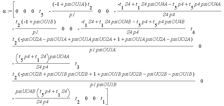
# By comparing with the vector th components, one will conclude that 11 parameters (the number of null components in alpha) are separately identifiable:
S1,S2,S3,psiOU2A,psiOU3A,psiOU2B,psiOU3B,psiUO3A,psiUO4A,psiUO3B,p2,p3
The other parameters
S4, psiOU1A, psiOU4A, psiOU1B, psiOU4B, psiUO1A, psiUO2A, psiUO4A, psiUO1B, psiUO2B, psiUO4B, p1 and p4
are not separately identifiable.
Indeed, the parameter psiOU1A (e.g.) cannot be estimated separately, because
at the fifth place in vector alpha there is an expression and not a 0.
If model {St, ,,
pt} would be used with real data, one would nevertheless get
an apparent estimate of psiOU1A. However, this estimate cannot be interpreted.
Actually, these 13 not separately identifiable parameters are functions of 19
� 11 = 8 (rank of A minus number of zeros in alpha) complex quantities.
These complex quantities are also estimable (see Gimenez
et al. 2003 for further details).
Literature cited Brownie, C., J. E. Hines, J. D.
Nichols, K. H. Pollock, and J. B. Hestbeck. 1993. Capture–recapture studies
for multiple strate including non-Markovian transitions. Biometrics 49:1173–1187.
Catchpole, E. A., and B. J. T. Morgan.
1997. Detecting parameter redundancy. Biometrika 84:187–196. Catchpole, E. A., B. J. T. Morgan,
and A. Viallefont. 2002. Solving problems in parameter redundancy using computer
algebra. Journal of Applied Statistics 29:625–636. Gimenez, O., R. Choquet, and J.-D.
Lebreton. 2003. Parameter redundancy in multistate capture-recapture models.
Biometrical Journal 45:704.