Martin Hoyle and James E. Creswell. 2007. The effect of wind direction on cross-pollination in wind-pollinated GM crops. Ecological Applications 17:1234–1243.

Appendix G. Correction to three-hourly wind data.

Method

Wind direction and speed was provided every hour and every three hours for the UK and European weather stations respectively. The total variance in pollen distribution () is given (Moore 1976) as

where and are the variances in pollen distribution due to diffusion, and to changes in wind direction within the sampling period respectively. The estimates of from Appendix C assume a 1-hour time interval between observations. Meteorological conditions are usually assumed roughly constant over a period of up to an hour (Hunt et al. 2001). We assume that the time that pollen is airborne is small compared to the time between wind direction readings (1 hour). Suppose pollen is moving downwind at low speed, say 1 ms^-1. Suppose further that we consider separation distances up to 1000 m. The time taken to travel 1000 m is 1000 s = 17 min < 1 hour. Hence we can assume that the wind direction does not change significantly over the period when a single pollen grain is airborne. Our aim was therefore to estimate for the European stations. Without this correction, we would underestimate for the European stations.

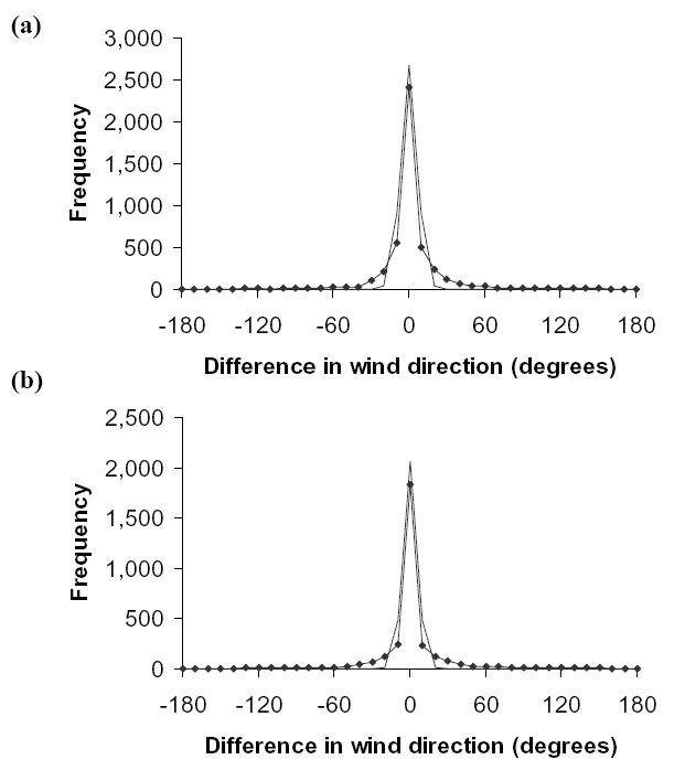
First, we estimated for the UK stations based separately on intervals of 1 and 3 hours. For each of the UK weather stations and years used in the analysis of the UK data, and for each hour between 9am and 6pm, the following four values were calculated: the difference in the wind direction at that hour and zero hours later (i.e., 0 degrees), the difference in the wind direction at that hour and one hour later, the difference in the wind direction at that hour and two hours later, and finally the difference in the wind direction at that hour and three hours later. The period from 9am to 6pm represents a typical period of pollen release. Data was calculated for the period 1st April to 30th September, the period over which all crops combined flowered. The first three differences above were combined, and the frequency of the differences in angles was calculated. The standard deviation of the normal distribution fitted to this frequency data ( (0,1,2 hours)) was estimated using the routine “Solver” in MS Excel (Microsoft Corp.), based on minimizing the residual sums of squares (Table G1a). The same procedure was applied to the differences in angles at zero hours and at three hours later to give (0,3 hours). As an example, the fits to normal distributions for the estimation of (0,1,2 hours) and (0,3 hours) for Perth for the year 1995 are given in Fig. G1. (0,3 hours) was then calculated in exactly the same way separately for all European stations and all years (Table G1b).

For the UK stations, (0,1,2 hours) and (0,3 hours) both vary little by sites and year, at about 6.5° and 6° respectively (Table G1a). Furthermore, (0,3 hours) also varies little among sites and years for the European stations, at approximately the same value as for the UK stations (Table G1b). For this reason, we set (0,1,2 hours) for the European stations as the same value as for the UK stations at 6°, independent of site and year.

Validation of method

The following procedure was performed to validate of the method of allowing for the variation in wind direction within 3 hours.

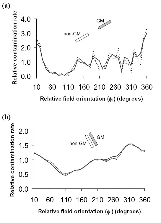
All data points were removed for the Nottingham 1998 dataset, except for those corresponding to the following times of day: 0:00, 3:00, 6:00, 9:00, 12:00, 15:00, 18:00 and 21:00. These times corresponded to those of the European stations. Relative cross-pollination rates for winter oilseed rape were then calculated separately on three bases;

• the reduced (3 hour) dataset with no adjustment for wind direction ( (0,1,2 hours) = 0°),
• the reduced (3 hour) dataset with adjustment for wind direction ( (0,1,2 hours) = 6°) and,
• the full (1 hour) dataset, separately for = 5°, 13° and 19°.

There were large differences between relative cross-pollination rates based on the reduced datasets without wind direction adjustment and the full datasets. There was little difference between relative cross-pollination rates based on the reduced datasets with wind direction adjustment and the full datasets, which gives visual confirmation of the validity of the method described above (Fig. G2). The greatest difference between the relative cross-pollination rates calculated on these two bases occurred for the smallest value of and for narrow distant fields. Nevertheless, the relative cross-pollination rates were still very similar (Fig. G2).

TABLE G1a. (0,1,2 hours) and (0,3 hours) for all UK stations and years.

TABLE G1b. (0,3 hours) for all European stations and years.

FIG. G1. Best fits to normal distributions for the estimation of (a) (0,1,2 hours) and (b) (0,3 hours) for Perth for the year 1995.

FIG. G2. Comparison of relative contamination rates for winter oilseed rape based on the reduced (3 hour) Nottingham 1998 dataset with no adjustment for wind direction (dotted line), the reduced datasets with adjustment for wind direction (narrow continuous line), and the full (1 hour) dataset (full continuous line), separately for (a) narrow distant fields, and (b) long close fields. = 5° in both cases.

LITERATURE CITED

Hunt, J. C. R., H. L. Higson, P. J. Walklate, and J. B. Sweet. 2001. Modelling the dispersion and cross-fertilisation of pollen from GM crops. Report to Department for Environment, Food and Rural Affairs.

Moore, D. J. 1976. Calculation of ground level concentration for different sampling periods and source locations. Atmospheric Pollutions. Elsevier, Amsterdam, 5160.