Pierre Legendre, Daniel Borcard, and Pedro Peres-Neto. 2005. Analyzing beta diversity: partitioning the spatial variation of community composition data. Ecological Monographs 75:435–450.

Appendix B. Partitioning examples: an explanation, a Table B1 and three Figures: Fig. B1, Fig. B2 and Fig. B3.

This appendix contains the analysis of one of the sets of data tables used in the simulation study. Readers will be able to examine a series of generated data tables, and appreciate the steps of the statistical analysis.

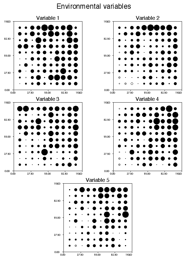
Two tables of species and one table of environmental data were generated using the stochastic procedure described in the "Data generation" subsection. The data sets contained 100 rows corresponding to 100 sites forming a 10 × 10 regular grid in the 100 × 100 field. Five environmental variables were generated, each one with a deterministic structure (gradient), autocorrelation controlled by a spherical variogram model with a range of 15, and standard normal deviates N(0,1) at each site. This example thus does not correspond to the simulations, where the environmental variables had either spatial autocorrelation or a deterministic structure, not both. The random normal deviates contributed 472 units to the sum of squares, the spatial autocorrelation component 482 units, and the deterministic slope 537 units, for a total sum of squares of 1491 in the environmental variables. These variables were normally distributed. Five species were created with random normal deviates plus autocorrelation (variogram with range = 15). Following Eq. 3, five more species were created, with random normal deviates, spatial autocorrelation, plus an effect of an environmental variable on each of the five species, with transfer parameter β = 0.5. The preliminary species were then transformed to species presence-absence or abundance data, as described in the "Data generation" subsection. The random N(0,1.5) constants multiplying the species to make their means different were –3.21, 2.07, –1.06, –3.39, 2.54, 1.68, –1.70, 1.44, 1.48, and 0.11. 50.4% of the entries in the two species files were zeros.

PCNM base functions were created using the program SpaceMaker2 (Borcard and Legendre 2004). We asked the program to create a regular (10 × 10) grid and used 1.4143 as the truncation distance, meaning that the west-east, south-north, and diagonal connections between adjacent points were preserved. In view of canonical partitioning, forward selection of PCNM base functions was carried out in Canoco v. 4.5 (ter Braak and Smilauer 2002). Nine PCNM variables were retained for each data set (species presence-absence and abundance, Hellinger-transformed), as shown in the notes of Table B1. Variation partitioning was done using a canonical partitioning program written by PL; identical results would have been obtained from simple and partial RDA in Canoco. Prior to Mantel-type partitioning, distance matrices were computed as described in the simulation study; Hellinger distances were computed for the two raw species data sets. Partitioning was conducted using the program Permute! version 3.4 (Casgrain 2001).

Supplement 2 contains the two raw species data files (Species_pres-abs.txt and Species_abund.txt), the same files after Hellinger transformation (Species_pres-abs_Hell.txt and Species_abund_Hell.txt) which were used to carry out the redundancy analyses reported in Table B1, the environmental data file (Envir.txt), the file with the geographic coordinates of the sites (CoordXY.txt), as well as the two files of PCNM base functions after forward selection (9_PCNMs_for_pres-abs.txt and 9_PCNMs_for_abundance.txt), as described in the previous paragraph.

The results for this data set illustrate the first result of the simulation study: compared to canonical partitioning, regression on distance matrices highly underestimates the portions of the species variation explained by the environmental variables alone (Table B1 columns [a+b]), the spatial relationships alone (columns [b+c]), or both sources of variation (columns [a+b+c]).

For the species abundance data, the partitioning results would have been very different without the Hellinger transformation. With the environmental variables and the 3rd-order polynomial of the geographic coordinates as explanatory variables, for example, the total portion of explained variation [a+b+c] would have been 0.1624 (fraction not significant, P = 0.254), while after Hellinger transformation of the abundance data [a+b+c] = 0.2014 (fraction significant, P = 0.002) as shown in Table B1. For presence-absence data, the result without Hellinger transformation ([a+b+c] = 0.2320, P = 0.001) would have been comparable to the one reported in Table B1 ([a+b+c] = 0.2276, P = 0.001) with Hellinger transformation. The Hellinger transformation has very little effect on this particular presence-absence data set because 75% of the sites have from 4 to 6 species present. If all the sites had the exact same number of species present, the Hellinger transformation would have no effect at all on the presence-absence canonical analysis results.

LITERATURE CITED

Borcard, D., and P. Legendre. 2004. SpaceMaker2 – User's guide. Département de sciences biologiques, Université de Montréal, Montréal, Canada.

Casgrain, P. 2001. Permute! version 3.4 – User's manual. Département de sciences biologiques, Université de Montréal, Montréal, Canada .

ter Braak, C. J. F., and P. Smilauer. 2002. Canoco reference manual and CanoDraw for Windows user's guide: software for canonical community ordination (version 4.5). Microcomputer Power, Ithaca, New York, USA.

TABLE B1. Example data: portion of the species variation in the fractions defined in Fig. 1. The environmental variables were included in all analyses, in the form of either a raw data table (RDA) or a distance matrix (Mantel). "Mantel" refers to regression on distance matrices.

Partitioning method	[a+b+c]	[a+b]	[b+c]	[a]	[b]	[c]	[d]
a) Species presence-absence
RDA, XY	0.15463	0.13843	0.06483	0.08983	0.0487	0.0162NS	0.8455
RDA, polynomial	0.22763	0.13843	0.15433	0.07332	0.0651	0.0892NS	0.7724
RDA, PCNM†	0.28803	0.13843	0.20433	0.08372	0.0548	0.14953	0.7121
Mantel, D(XY)	0.01843	0.01813	0.00461	0.01392	0.0042	0.0004NS	0.9816
Mantel, D(polyn.)	0.01833	0.01813	0.00441	0.01392	0.0041	0.0003NS	0.9817
Mantel, ln(D(XY))	0.01913	0.01813	0.00552	0.01352	0.0045	0.0010NS	0.9809
b) Species abundance
RDA, XY	0.11972	0.09823	0.05152	0.0682NS	0.0300	0.0215NS	0.8803
RDA, polynomial	0.20142	0.09823	0.14143	0.0600NS	0.0382	0.1033NS	0.7986
RDA, PCNM‡	0.26663	0.09823	0.19663	0.07001	0.0282	0.16843	0.7334
Mantel, D(XY)	0.00692	0.00612	0.00312	0.00381	0.0023	0.0009NS	0.9931
Mantel, D(polyn.)	0.00702	0.00612	0.00332	0.00371	0.0024	0.0009NS	0.9930
Mantel, ln(D(XY))	0.00773	0.00612	0.00402	0.00371	0.0024	0.00161	0.9923

Notes:

† 9 PCNM base functions were retained by forward selection (Canoco 4.5) at P ≤ 0.05: PCNM #1, 3, 4, 6, 9, 16, 41, 42, 57.

‡ 9 PCNM base functions were retained by forward selection (Canoco 4.5) at P ≤ 0.05: PCNM #1, 5, 6, 10, 12, 26, 42, 44, 57.

Significance of the fractions (permutation tests, 999 permutations): ¹ 0.01 < P ≤ 0.05, ² 0.001 < P ≤ 0.01, ³ P ≤ 0.001, ^NS not significant (P > 0.05). Fractions [b] and [d] cannot be tested for significance.

FIG. B1. Values of the five environmental variables at 100 sampling sites on the 10 × 10 regular grid positioned in a 100 × 100 field (arbitrary units). Each variable was generated independently of the others; it contains a deterministic structure (gradient), spatial autocorrelation, and random "innovation" at each site. Dark circles: positive values; empty circles: negative values.

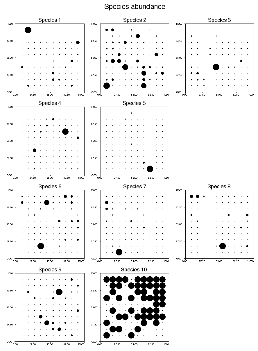
FIG. B2. Species abundance (not Hellinger-transformed) at the 100 sampling sites on the 10 × 10 regular grid positioned in a 100 × 100 field (arbitrary units). Species 1 to 5 are only structured by spatial autocorrelation plus random error; species 6 to 10 are also related to the environmental variables shown in Fig. B1. Raw abundances, before Hellinger transformation. Dark circles: positive values; empty circles: negative values. Bubble sizes are standardized within each graph. They are comparable within a species map but not among maps. Because of its small multiplier, species 10 only contains 0's (49%) and 1's (51%).

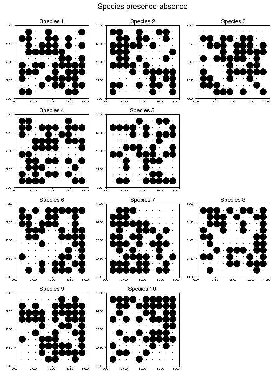
FIG. B3. Species presence-absence data at the 100 sampling sites on the 10 × 10 regular grid positioned in a 100 × 100 field (arbitrary units). Dark circles: species present; points: species absent. Patchiness due to autocorrelation in present in all species. The effect of the gradient present in the environmental variables is visible in the distributions of species 6 to 10, which are each related to one of the environmental variables by a transfer parameter β = 0.5.