Ecological Archives M085-021-A2

Stephen J. Tulowiecki and Chris P. S. Larsen. 2015. Native American impact on past forest composition inferred from species distribution models, Chautauqua County, New York. Ecological Monographs 85:557–581. http://dx.doi.org/10.1890/14-2259.1

Appendix B. A brief introduction into cost-distance analyses, and the steps taken to create Native American variables (NAVs).

This appendix provides a brief introduction into cost distance modeling, and then presents the three steps taken to create Native American variables (NAVs) for this study. The NAVs developed in this study were the following: accessibility to a Historic Iroquoian village site, accessibility to a Late Woodland Iroquoian village site, and accessibility to an Iroquoian trail.

Cost-distance analyses, along with least-cost path analyses, have been used throughout archaeology and anthropology (Surface-Evans and White 2012). Often aided by GIS, the basic goals of such analyses are to understand past patterns of human movement and landscape use. Cost-distance analyses first require the calculation of a “cost surface” or “friction surface,” in order to represent the ease or difficulty of travel per unit distance, given a set of environmental or physiological constraints. Common environmental variables that affect the human physiological cost of movement through an analysis cell can include topography (i.e., slope angle), land cover, and hydrography (Howey 2011). Researchers have more recently modeled energy expenditure of human foot-travel, using data from studies of human physiology (White and Barber 2012). Applications of cost-distance analyses include the modeling of least-cost paths between archaeological sites (Nolan and Cook 2012), and the calculation of resource catchments surrounding archaeological sites based upon modeled energy expenditure (Verhagen and Whitley 2012).

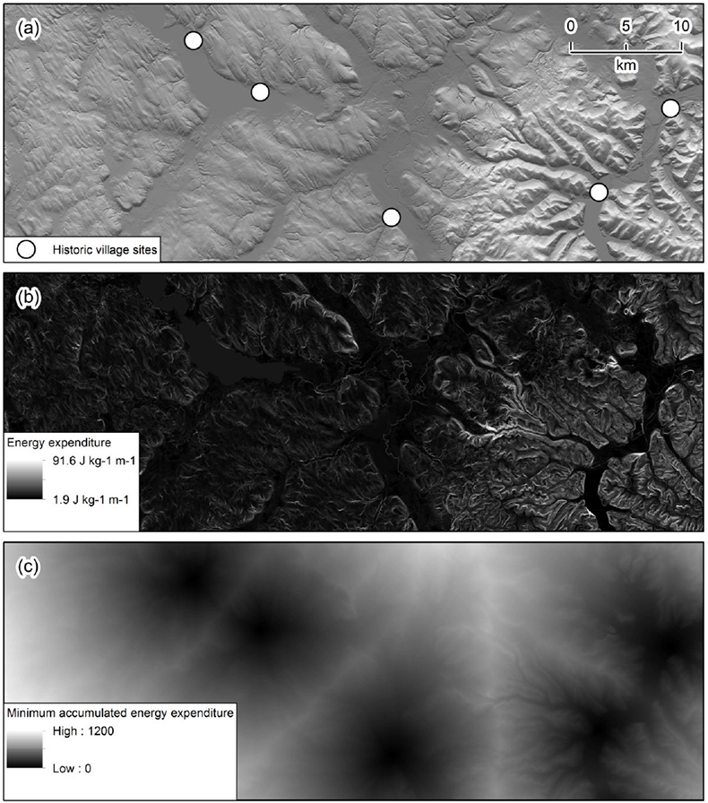
Modeling the minimum accumulated energy expenditure for each NAV required three steps, and was performed at a 10 × 10 m rid cell resolution and later mean-aggregated to 100 × 100 m using ArcGIS tools (Esri 2012). The steps were based upon the methods of Jobe and White (2009), who modeled energy expenditure as a function of terrain slope angle, stream crossings, and other variables. First, a cost surface (Fig. B1b), which represented the energy that would be expended (in J kg-1 m-1) as a function of terrain slope angle, was calculated for each grid cell using the published findings of Minetti et al. (2002). The Minetti et al. (2002) study related slope angle to energy expenditure at walking speed, using treadmill experiments. Because energy expenditure due to slope angle is not isotropic with respect to the direction of travel (e.g., walking down a modest slope requires less energy than walking the same slope uphill), energy expenditure was calculated to represent an average of both inbound and outbound travel through each cell. To calculate energy expenditure resulting from slope angle in each cell, two second-order polynomials were fitted separately to the data of Minetti et al. (2002), to model the relationship between slope angle and energy expenditure:

In the above equations, x equals slope angle in degrees, and y equals energy expenditure for a person, in J·kg^-1·m^-1. The polynomials also extrapolated energy expenditure to slope angles of ±30°; Minetti et al. (2002) tested slope angles up to ±24°. About 0.6% of the study area exceeded 24° in slope angle at 100 × 100 m resolution. Using Raster Calculator (Esri 2012) and a slope raster, one calculation for energy expenditure through each cell was made using each polynomial above, and the two calculations were then averaged together. These calculations were not made for Lake Erie and Chautauqua Lake, and cells within these water bodies were assigned a constant value based upon typical energy expenditure for canoe travel (The United States Army 2007).

The second step was to modify the energy expenditure calculations in the previous step, to account for additional landscape factors upon energy expenditure. Soule and Goldman (1972) developed coefficients (using field and treadmill experiments) to represent the multiplicative effects upon energy expenditure, from foot-travel over conditions such as gravel roads (coefficient = 1.1), light brush (coefficient = 1.2), heavy brush (coefficient = 1.5), and swampy terrain (coefficient = 1.8). Using the coefficients of Soule and Goldman as a guide, four coefficients were estimated to modify the energy expenditure calculations in the first step. A coefficient of 1.2 was assigned to areas with soils that were either somewhat excessively well-drained, or well-drained (Natural Resources Conservation Service 2013). A coefficient of 1.5 was assigned to areas with soils that were moderately well-drained, or somewhat poorly drained. These coefficients were estimated to represent the potential difficulties of traveling through muddy or waterlogged soils. A coefficient of 1.8 was assigned to areas with soils that were poorly drained or very poorly-drained; these areas corresponded well with swampy areas within the study area. Using ArcHydro tools (Esri 2012), stream networks were mapped, and streams were assigned a coefficient of 1.8 to represent a “penalty” for stream crossing. Iroquoian trails were not assigned a coefficient that made travel easier, because the contemporaneity of trails with villages was unknown. In order to create the final cost surface, the raster layer that represented energy expenditure due to slope factors, was multiplied by a raster layer representing the coefficients designated above.

The third and final step was to use the cost surface to calculate minimum accumulated energy expenditure to each cell within the study area, from village sites or trails (Fig. B1a, c). The cost surface was inputted into the “Path Distance” tool in ArcGIS (Esri 2012), which calculated the minimum possible cost (in J/kg) to access each cell from a feature. A DEM was also inputted into the tool, to model energy expenditure in a manner that considered distances traveled over three-dimensional terrain. One calculation was made for each NAV, in order to calculate the minimum possible energy expenditure to a Late Woodland village site, Historic village site, or trail. The calculations for each NAV were converted from J/kg, to kcal for a 70 kg person, in order to enhance the interpretability of the variables (e.g., how much energy a person weighing 70 kg would expend, by traveling from a trail or village site). One mid-19th century report indicated that the average weight of Native American males living on western New York reservations was 73.8 kg (Hauptman 1993).

Fig. B1. An example of how “accessibility to a Historic village site” was calculated. A portion of the Historic village sites is depicted on a relief map in (a). The first two steps involved creating a cost surface, depicted in (b). This cost surface represented the per-unit energy expenditure for traveling across a cell, based on factors such as slope. Using the cost surface, the third step calculated minimum accumulated energy expenditure to a Historic village site, as depicted in (c).

Literature cited

Esri. 2012. ArcGIS 10.1. Redlands, CA, USA.

Hauptman, L. M. 1993. The Iroquois and the Civil War: From Battlefield to Reservation. Syracuse University Press, Syracuse, NY, USA.

Howey, M. C. L. 2011. Multiple pathways across past landscapes: circuit theory as a complementary geospatial method to least cost path for modeling past movement. Journal of Archaeological Science 38:2523–2535.

Jobe, R. T., and P. S. White. 2009. A new cost-distance model for human accessibility and an evaluation of accessibility bias in permanent vegetation plots in Great Smoky Mountains National Park, USA. Journal of Vegetation Science 20:1099–1109.

Minetti, A. E., C. Moia, G. S. Roi, D. Susta, and G. Ferretti. 2002. Energy cost of walking and running at extreme uphill and downhill slopes. Journal of Applied Physiology 93:1039–1046.

Natural Resources Conservation Service. 2013. Geospatial Data Gateway. United States Department of Agriculture. Available at: http://datagateway.nrcs.usda.gov/.

Nolan, K. C., and R. A. Cook. 2012. A method for multiple cost-surface evaluation of a model of Fort Ancient interaction. Pages 67–93 in S. L. Surface-Evans and D. A. White, editors. Least cost analysis of social landscapes: archaeological case studies. The University of Utah Press, Salt Lake City, UT USA.

Soule, R. G., and R. F. Goldman. 1972. Terrain coefficients for energy cost prediction. Journal of Applied Physiology 32:706–708.

Surface-Evans, S. L., and D. A. White. 2012. An introduction to the least cost analysis of social landscapes. Pages 1–10 in S. L. Surface-Evans and D. A. White, editors. Least cost analysis of social landscapes: archaeological case studies. The University of Utah Press, Salt Lake City, UT USA.

The United States Army. 2007. Army field manual FM 21-20 (physical fitness training). Headquarters, Department of the Army, Washington, DC, USA.

Verhagen, P., and T. G. Whitley. 2012. Integrating archaeological theory and predictive modeling: a live report from the scene. Journal of Archaeological Method and Theory 19:49–100.

White, D. A., and S. B. Barber. 2012. Geospatial modeling of pedestrian transportation networks: a case study from precolumbian Oaxaca, Mexico. Journal of Archaeological Science 39:2684–2696.

[Back to M085-021]