Ecological Archives M085-015-A1
Chengjin Chu and Peter B. Adler. 2015. Large niche differences emerge at the recruitment stage to stabilize grassland coexistence. Ecological Monographs 85:373392. http://dx.doi.org/10.1890/14-1741.1
Appendix A. The influence of individual plant buffer width on our results.
Our algorithm for tracking survivors and new recruits in the historical mapped quadrats involves setting a “buffer width,” the distance a genet can move between years and still retain its original identity. The choice of buffer width does influence vital rates: a larger buffer width means that a polygon is more likely to be classified as a survivor than a new recruit, and thus tends to increase mean survival rates and decrease mean recruitment rates. Here we (1) provide an example to illustrate why we add a buffer around each polygon when extracting demographic data, (2) repeat our analysis of invasion growth rates and simulated equilibrium cover for the extreme case of a buffer = 0 cm, and (3) show that our qualitative conclusion about niche differences and average fitness differences does not appear sensitive to the choice of buffer width.
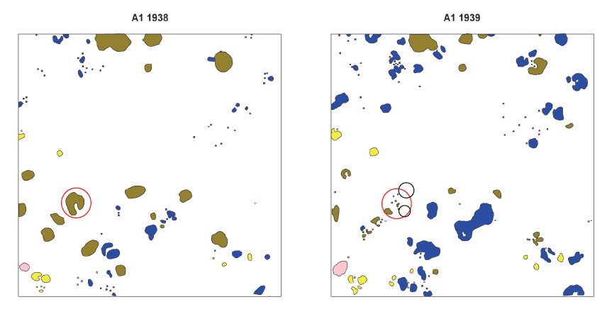
1.1. To illustrate how the buffer width affects our genet tracking algorithm, we focus on a quadrat A1 at the Montana study site (NMP, MT) in 1938 and 1939 (Fig. A1). Different colors represent different species. The red circle marks a large genet in 1938 that fragments in 1939, at the height of the Great Drought. If we apply a 5 cm buffer, all the small polygons falling within the red circle in 1939 retain the same genet identity. If we set the buffer to zero, two polygons in 1939 (such as the two small black circles) would be labeled as new recruits. Note that traditional plant demography studies, which rely on tags to mark individual plants, face the same problem of determining the identity of stems that “move” small distances from year to year.
Fig. A1. An example to illustrate why we add a buffer around each polygon when extracting demographic data.
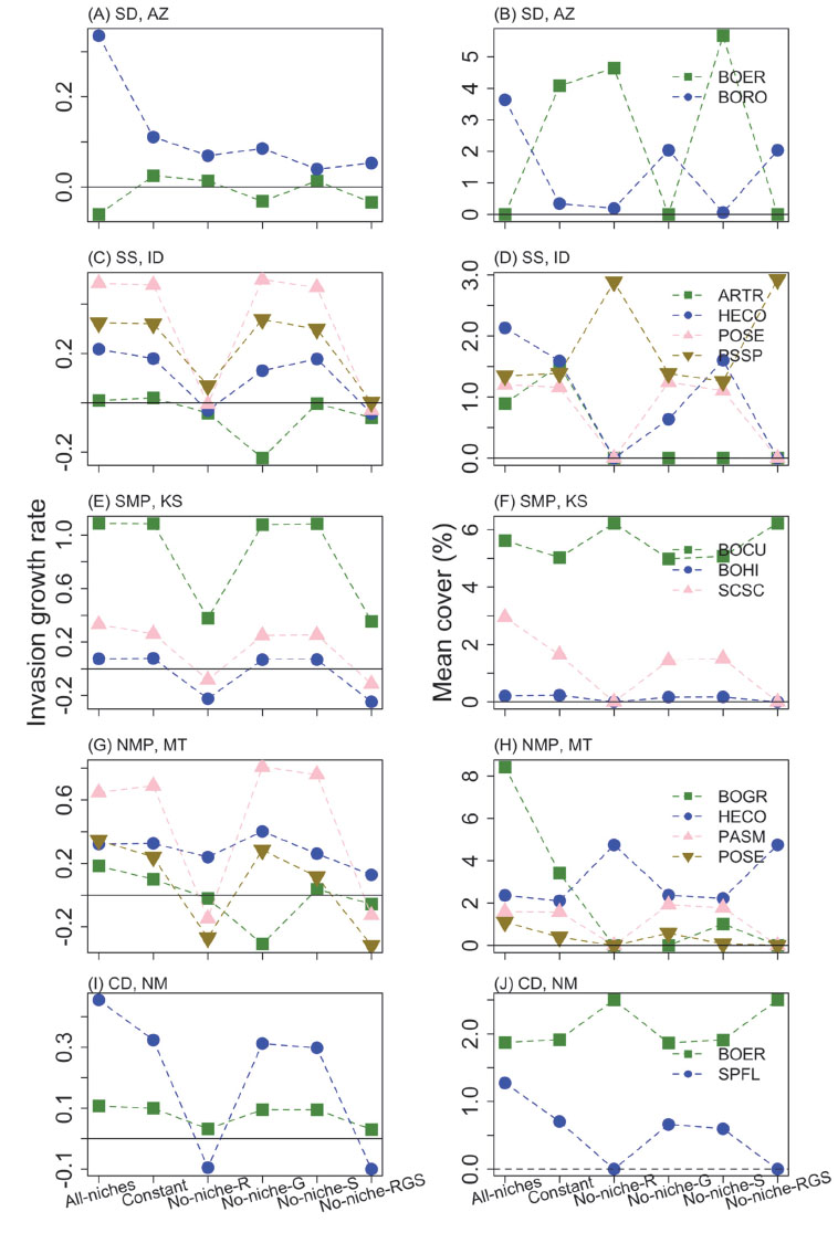
1.2. We repeated our analysis, from beginning to end, with the buffer width set = 0 cm. The following figures can be compared directly to Fig. 5. Each figure shows the invasion growth rates (left column) and average cover (right column) simulated by the IPM models for each study site, for the following models: observed parameters without any perturbation (‘All-niches’), a constant environment (‘Constant’), and a constant environment with stabilizing mechanism removed from recruitment (‘No-niche-R’), growth (‘No-niche-G’), survival (‘No-niche-S’), or all three vital rates (‘No-niche-RGS’). The two study species in SD, AZ did not coexist in the All-niches model built from data based on a buffer of 0 cm (i.e., the negative invasion growth rate for species BOER with the cover of zero). See the section Summary of study sites and species selection in Materials and Methods for the abbreviations for species names.
Consistent with the results from the case with the buffer = 5 cm, removal of temporal fluctuations did not remarkably alter the invasion growth rates or species’ cover at equilibrium, and removing stabilization mechanisms from recruitment (‘No-niche-R’) always led to the greatest reduction in invasion growth rates on average.
Fig. A2. The result of our analysis of invasion growth rates and simulated equilibrium cover for the extreme case of a buffer = 0 cm.
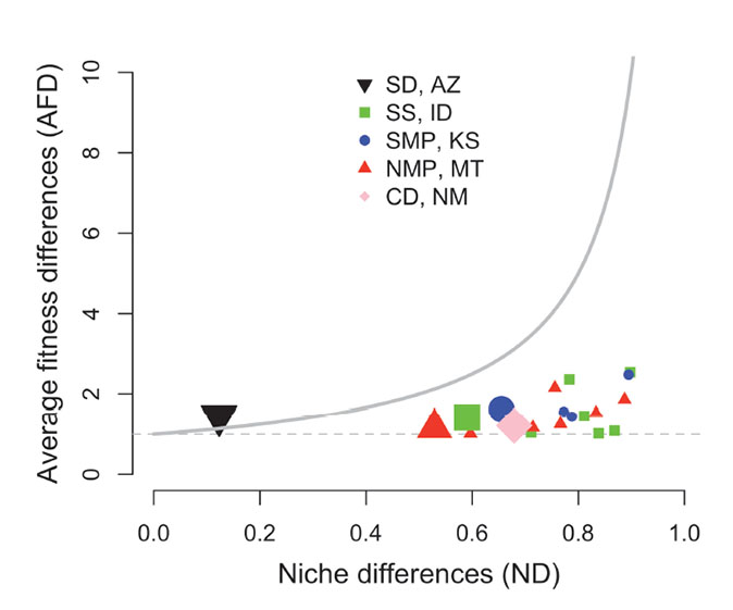
1.3. We also repeated the pairwise species invasion simulations necessary to use Carroll et al’s. formula for estimating niche differences and average fitness differences. Fig. A3, based on data extracted using buffer = 0 cm, can be compared directly to Fig. 5. Smaller symbols represent the niche differences (ND) and average fitness differences (AFD) for species pairwise comparisons from five study sites. The community-level ND and AFD for each study site are represented by the larger symbols. For Arizona and New Mexico, sites with only two species modeled, the pairwise and the community-level ND and AFD are equivalent. Competitive exclusion occurs above and to the left of the curve, AFD=1/(1-ND), and coexistence occurs below and to the right. AFD with the value of 1 (dashed line) means no fitness differences existing between species.
The results showed that four of five communities displayed similar patterns as for the 5-cm buffer case. The exception came from the SD community in Arizona, where B. eriopoda could not persist in the zero buffer case, supporting our contention that a non-zero buffer around each polygon is more realistic.
Fig. A3. Niche differences (ND) and average fitness differences (AFD) for 17 species pairs (smaller symbols) from five study sites for the extreme case of a buffer = 0 cm. The community-level ND and AFD for each study site were represented by the larger symbols.