Ecological Archives M082-123-A2

Brett T. McClintock, Ruth King, Len Thomas, Jason Matthiopoulos, Bernie J. McConnell, and Juan M. Morales. 2012. A general discrete-time modeling framework for animal movement using multi-state random walks. Ecological Monographs 82:335–349. http://dx.doi.org/10.1890/11-0326.1

Appendix B. Reversible jump Markov chain Monte Carlo algorithm for the multi-state random walk model.

The multi-state biased correlated random walk model is particularly well suited to a Bayesian analysis utilizing Markov chain Monte Carlo (MCMC) methods. With c centers of attraction and h exploratory states, one can implement a MCMC algorithm for the parameters of the movement process model as follows:

(1) Initialize all parameters (including the latent state vector ). Start the chain at iteration g = 1.

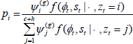
(2) For each iteration g, use a Gibbs step to update = {1, ..., c + h} for t = 1, ..., T by drawing a categorical random variable from the full conditional distribution. For the simplest model assuming independence, the full conditional distribution (given all other parameters and random variables) is:

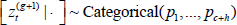
where:

For a first-order Markov switching model, an initial latent state z₀ must also be included. Assuming each state is equally likely a priori, is first updated from its full conditional distribution:

where:

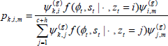
The full conditional distribution for t = 1, ..., T is:

where:

(3) Update the state transition probabilities ψ^(g) using a Gibbs step. With prior distribution ψ ~ Dirichlet(α₁ + v₁, ..., α_c + h) for the simplest model assuming independence,

where:

With prior distribution ψ_k ~ Dirichlet(α_k, 1, ..., α_{k, c + h}) for a first-order Markov switching model,

for k = 1, ..., c + h where .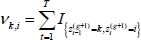

(4) Update for z = {1, ..., c} using a random walk Metropolis-Hastings (MH) step. Propose a new value from some distribution with probability density function q(|) and accept the proposed value with probability:

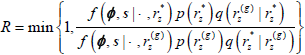
where p(r_z) is the prior distribution density for r_z. If the proposed value is accepted, set = . Otherwise, set = . If applicable, use a similar random walk MH step for intercept (m_z), quadratic (q_z), or higher-order terms.

(5) Update the center of attraction correlation parameter η_z for for z = {1, ..., c} using a random walk MH step.

(6) Update the exploratory state correlation parameters v_z for z = {c + 1, ..., c + h} using a random walk MH step.

(7) Update the initial movement direction parameter φ₀ using a random walk MH step.

(8) Update the locations for each of the c centers of attraction () for z = {1, ..., c} using a random walk MH step. Propose new location for center of attraction z() from some distribution with probability density function q( | ). Propose = {1, ..., c + h} for t = 1, ..., T using the full conditional distribution from step 2 above, and accept the proposed values with probability:

where p(z) and q(z) are the respective prior and proposal densities for z. If the proposed values are accepted, set
() = () and = for t = 1, ..., T. Otherwise, set () = () and = for t = 1, ..., T.

(9) Block update scale a_z and shape b_z parameters for z = {1, ..., c + h} and step length change-point distance d_z parameters for z = {1, ..., c} using a random walk MH step.

(10) Increment g by 1 and return to step 2.

When using a state-space formulation, one can implement a MCMC algorithm for the observation model parameters as follows:

(1) Initialize all parameters. Start the chain at iteration g = 1.

(2) Block update coordinates of regular locations (,) for t = 0, ..., T using a random walk MH step. Propose new values and from some distributions with respective probability density functions q(|) and q(|), and accept with probability

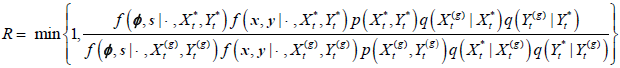
where f(x, y|-, X_t, Y_t) is the likelihood function for the observation model and p(X_t, Y_t) is the joint prior distribution for X_t and Y_t If the proposal is accepted, set () = (,). Otherwise, set () = (,)

(3) Update measurement error parameters (e.g., and ) using single update random walk MH steps.

(4) Increment g by 1 and return to step 2.

Switching from one movement process model to another generally involves adding or removing parameters within each iteration of the Markov chain. This can be achieved using a reversible jump Markov chain Monte Carlo algorithm (e.g., Green 1995, Richardson and Green 1997). Within each iteration of the Markov chain, three different movement model updates are proposed. These correspond to the quadratic bias towards centers of attraction (q_z) for z = {1, ..., c}, the correlations between successive movements for center of attraction states (η_z) for z = {1, ..., c} , and the correlation between successive movements for exploratory states (v_z) for z = {c + 1, ..., c + h}.

We cycle through the center of attraction and exploratory parameters in turn, performing each RJMCMC update as single steps. For center of attraction states z = {1, ..., c}, if q_z is present in the current model M^(g), we simply propose to remove it from proposed model M^*. If q_z is not present in M^(g), we propose to add it to M^*. Similarly, if η_z is present in M^(g), we propose to remove it from M^*. If η_z is not present in M^(g), we propose to add it to M^*. For exploratory states z = {c + 1, ..., c + h}, if v_z is present in M^(g), we propose to remove it from model M^*. If v_z is not present in M^(g), we propose to add it to M^*.

For illustration, suppose we are updating the bias relating to center of attraction 1, and that the current model, M^(g), only has the linear term (r₁) present. We then propose to add the quadratic term to model M^* and propose a new value

using the N(0, τ²) prior distribution as the proposal distribution. This model move is accepted with probability,

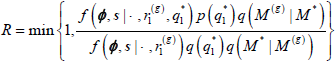
where q(M^*|M^(g)) denotes the probability (= 1) of proposing the quadratic model M^* given in linear model M^(g), and q(M^(g)|M^*) denotes the probability (= 1) of proposing the linear model M^(g) given in quadratic model M^*. If the model move is accepted, set
M^(g + 1) = M^*. Otherwise, set M^(g + 1) = M^(g). For the reverse model move, we propose to remove the quadratic term from model M^*. We accept this move with probability

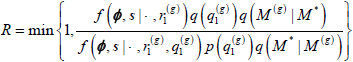
where q(M^(g)|M^*) = 1 and q(M^*|M^(g)) = 1. We use the analogous reversible jump updates on the correlation terms for center of attraction η_z and exploratory v_z states by using the Unif(0,1) priors as proposal distributions when proposing to add or remove these parameters.

By performing these model updates at each iteration, posterior model probabilities can be estimated as the proportion of iterations the Markov chain spends in each of the possible models. Monte Carlo estimates (including model-averaged estimates) may also be obtained for each of the parameters from this single Markov chain.

Green, P. J. 1995. Reversible jump Markov chain Monte Carlo computation and Bayesian model determination. Biometrika 82:711–732.

Richardson, S., and P. J. Green. 1997. On Bayesian analysis of mixtures with an unknown number of components. Journal of the Royal Statistical Society B 59:731–792.