Ecological Archives C006-055-A3

Ecological Archives C006-055-A3

Marcos Texeira, Mariano Yarzabal, Gervasio Pineiro, Santiago Baeza, and Jose Maria Paruelo . 2015. Land cover and precipitation controls over long-term trends in carbon gains in the grassland biome of South America. Ecosphere 6:196. http://dx.doi.org/10.1890/es15-00085.1

Appendix C. Trends in integrated precipitation use efficiency and precipitation marginal response.

In this appendix we show the results of the trend analyses for 3 and 5 year integrated precipitation use efficiency. We also show the patterns of precipitation marginal response for the subset of 12 ground meteorological stations with precipitation records from 1948 to 2011 and fPAR estimates from 1981 to 2011.

Table C1. Results of the regressions of 3 year integrated precipitation use efficiency against time for twelve sites with precipitation and fPAR records for the period 1981 to 2011. For each site the most parsimonious models according to Akaike information criterion is shown. “b1” represents the slope of the simple linear model and “p-val” the p value associated. Latitude (Lat) and longitude (Long) of sites are shown.

Site	b1	p	AIC	Lat	Long
S1) Baltasar Brum	-0.0028	0.868	15.998	30º43’30’’S	57º19’30’’W
S2) Queguay chico	-0.0060	0.596	7.985	32º4’30’’S	56º52’30’’W
S3) Paysandú	0.0159	0.500	12.993	32º22’30’’S	58º4’30’’W
S4) Treinta y Tres	0.0016	0.901	10.647	33º10’30’’S	54º22’30’’W
S5) Mercedes	-0.0016	0.907	11.798	33º16’30’’S	58º4’30’’W
S6) Trinidad	-0.0012	0.882	0.821	33º34’30’’S	56º52’30’’W
S7) Nueva Palmira	-0.0237	0.112	11.698	33º52’30’’S	58º22’30’’W
S8) Cerro Colorado	0.0079	0.636	15.693	33º52’30’’S	55º34’30’’W
S9) Estanzuela	0.0386	0.060	17.455	34º13’30’’S	57º25’30’’W
S10) Florida	0.0260	0.104	13.113	34º19’30’’S	56º16’30’’W
S11) Rocha	0.0342	0.072	16.150	34º31’30’’S	54º19’30’’W
S12) Libertad	0.0006	0.972	16.431	34º40’30’’S	56º34’30’’W

Table C2. Results of the regressions of 5 year integrated precipitation use efficiency against time for twelve sites with precipitation and fPAR records for the period 1981 to 2011. For each site the most parsimonious models according to Akaike information criterion is shown. “b1” represents the slope of the simple linear model and “p-val” the p value associated. Latitude (Lat) and longitude (Long) of sites are shown.

Site	b1	p	AIC	Lat	Long
S1) Baltasar Brum	-0.0099	0.519	5.808	30º43’30’’S	57º19’30’’W
S2) Queguay chico	-0.0120	0.479	7.020	32º4’30’’S	56º52’30’’W
S3) Paysandú	0.0156	0.424	4.430	32º22’30’’S	58º4’30’’W
S4) Treinta y Tres	-0.0064	0.657	5.388	33º10’30’’S	54º22’30’’W
S5) Mercedes	-0.0035	0.831	7.096	33º16’30’’S	58º4’30’’W
S6) Trinidad	-0.0080	0.250	-4.266	33º34’30’’S	56º52’30’’W
S7) Nueva Palmira	-0.0267	0.066	2.564	33º52’30’’S	58º22’30’’W
S8) Cerro Colorado	-0.0031	0.891	11.948	33º52’30’’S	55º34’30’’W
S9) Estanzuela	0.0319	0.238	11.846	34º13’30’’S	57º25’30’’W
S10) Florida	0.0175	0.434	10.190	34º19’30’’S	56º16’30’’W
S11) Rocha	0.0312	0.130	7.791	34º31’30’’S	54º19’30’’W
S12) Libertad	-0.0039	0.809	6.800	34º40’30’’S	56º34’30’’W

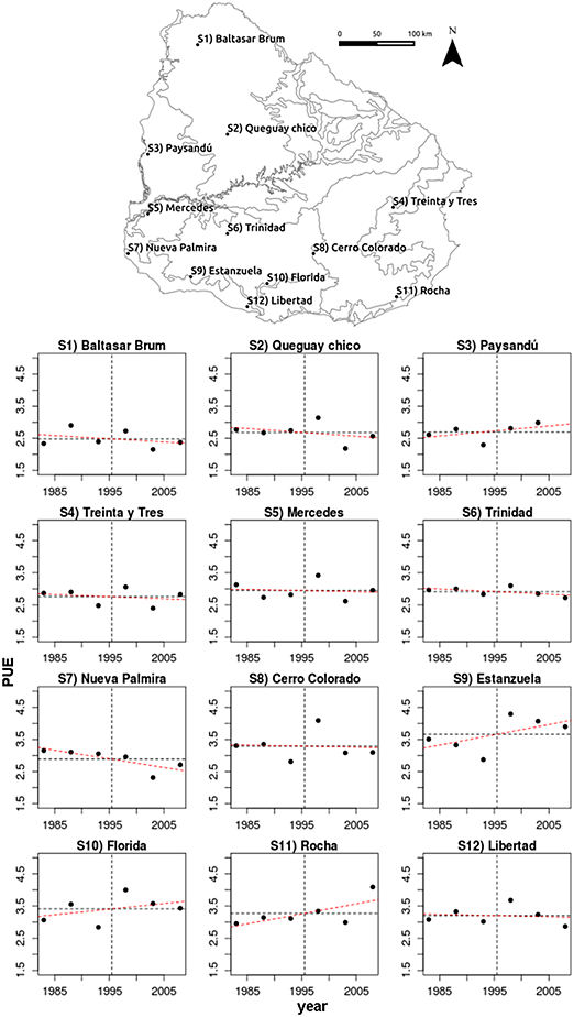
Fig. C1. Trends in 3 year integrated precipitation use efficency ((I-fPAR/accumulated precipitation) × 1000) for the period 1980–2011. Red broken lines represent best fit models (selected by means of AIC). Vertical broken lines represent the period mean whereas horizontal broken lines represent the mean PUE. All models were non significant at α=0.05.

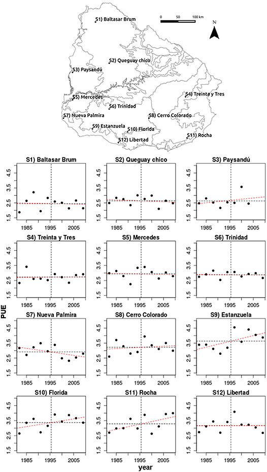
Fig. C2. Trends in 5 year integrated precipitation use efficency ((I-fPAR/accumulated precipitation) × 1000) for the period 1980-2011. Red broken lines represent best fit models (selected by means of AIC). Vertical broken lines represent the period mean whereas horizontal broken lines represent the mean PUE. All models were nonsignificant at α=0.05.

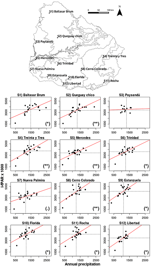
Fig. C3. Annually integrated fPAR × 1000 vs. annual precipitation for the period 1980–2011. The slopes associated to the red lines represent the precipitation marginal response (PMR). Slopes significant at an α = 0.01 are marked with (**), whereas those significant at an α = 0.05 are marked with (*).

[Back to C006-055]