Ecological Archives C006-054-A1

Mirjana Bevanda, Emanuel Fronhofer, Marco Heurich, Jörg Müller, and Björn Reineking. 2015. Landscape configuration is a major determinant of home range size variation. Ecosphere 6:195. http://dx.doi.org/10.1890/es15-00154.1

Appendix A. Additional information explaining the statistical models with figures and tables, in specific, the area dependencies of landscape indices, the home range size of red and roe deer across spatio-temporal scales, table of random effects for mixed models on all spatio-temporal scales for red and roe deer, and tables of the mixed models with different correlation structure for all spatio-temporal scales for red and roe deer.

Area dependencies of landscape indices

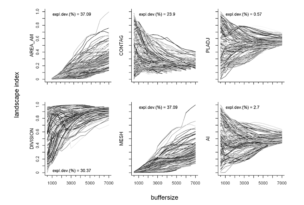
Buffers around 90% kernel home range centers (monthly scale, n = 214) from the red deer data set were drawn from 500 m to 7000 m in 500 m steps. We then calculated six landscape indices for each buffer circle (area–weighted mean patch area (AREA_AM), contagion (CONTAG), percentage of like adjacencies (PLADJ), landscape division index (DIVISION), effective mesh size (MESH), aggregation index (AI)). Afterwards we ran a mixed model to check for size dependencies of the indices. In total 13.42 % of calculated buffers were excluded from further analyses as they contained more than 5 % missing values in land cover data.

The analysis of the area–dependency of the landscape indices revealed a high size–dependency of the metrics AREA_AM, DIVISION and MESH, hence these indices were excluded from further analyses. Additionally the indices CONTAG, PLADJ, and AI were highly correlated with each other (Pearson’s correlation Index > 0.8). The PLADJ index accounts not only for patch size but also on patch shape (McGarigal et al., 2002), and furthermore shows the least dependency on area (Fig. 1), so we choose this index for all further analysis. Note that the indices AI and CONTAG show essentially the same results. The software tools R version 3.0.2 (R Development Core Team, 2013), GRASS 6.4.1 (Grass Development Team, 2012) and FRAGSTATS v3 (McGarigal et al., 2002) were used for the analyses.

Fig. A1. Overview of the size dependencies of six calculated landscape metrics analyzed with a mixed model. Buffer index values belonging to the same home range centre point are connected with a line. The explanatory value (expl.dev( %)) of the size dependency for each landscape index is drawn within the plot.

Home range size of red and roe deer across spatio–temporal scales

Table A1. Summary statistics of male and female red (A) and roe deer (B) home range sizes (km) across spatio–temporal scales (N = Number of samples included in home range estimation). Home ranges were estimated with the fixed kernel method using the reference method for the smoothing factor h (Worton, 1989; Kernohan et al., 2001). The software R version 3.0.2 using the package “adehabitatHR” was used for the analysis (R Development Core Team 2013, Calenge 2006).

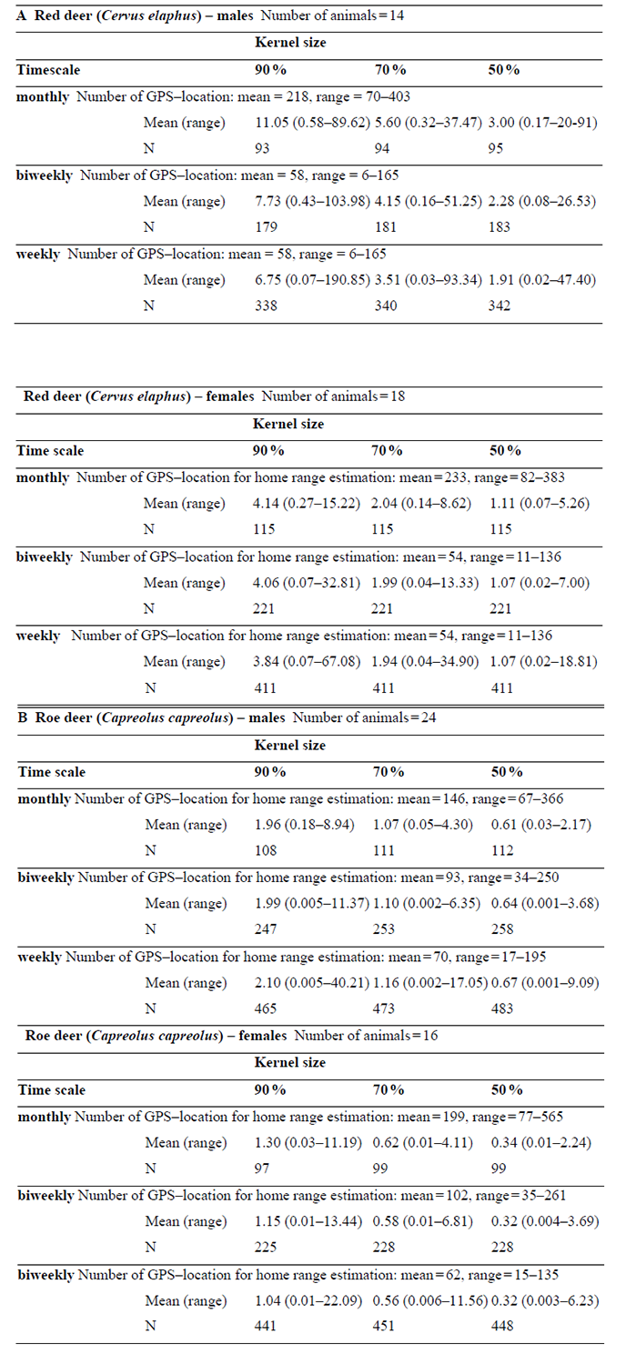
Table of random effects for mixed models on all spatio–temporal scales for red and roe deer

Table A2. Table of random effects and standard deviation (SD) of the linear mixed models for all spatio–temporal scales for both species, red (A) and roe deer (B). All models were fitted with ID as random effect. Additionally as the data samples are taken over different years, the models were additionally fitted with year as a nested variable within ID.

Tables of the mixed models with different correlation structure for all spatio–temporal scales for red and roe deer

We checked for spatial and temporal correlation structure using the full model. Following the approach of Borger (2006) we specified the spatial correlation structure with the geographic coordinates of the home range centers and used a vector for the temporal autocorrelation specifying the time variable. Afterwards we compared the models using the Akaike Information Criterion (AIC) to obtain the best model.

Table A3. Table of the red deer data set fitted with a mixed effect model with different correlation structure. The best models are indicated in bold format.

Table A4. Table of the roe deer data set fitted with a mixed effect model with different correlation structure. The best models are indicated in bold format.

Literature cited

Calenge, C. 2006. The package "adehabitat" for the R software: a tool for the analysis of space and habitat use by animals. Ecological Modelling 197:516–519.

Grass Development Team. 2012. Geographic Resources Analysis Support System (GRASS) Software, Version 6.4.1. http://grass.osgeo.org.

Kernohan, B. J., R. A. Gitzen, and J. J. Millspaugh. 2001. Analysis of animal space use and movements. In J. J. Millspaugh and J. Marzluff, editors, Radio Tracking and Animal Populations, pages 126–164. Academic Press, San Diego, California, USA.

McGarigal, K., S. Cushman, M. Neel, and E. Ene. 2002. FRAGSTATS v3: Spatial Pattern Analysis Program for Categorical Maps. Computer software program produced by the authors at the University of Massachusetts, Amherst.

R Development Core Team, 2011. R: A Language and Environment for Statistical Computing. R Foundation for Statistical Computing. http://www.r–project.org.

Worton, B. 1989. Kernel methods for estimating the utilization distribution in home-range studies. Ecology 70:164–168.

[Back to C006-054]