Ecological Archives E096-280-A1
Timothy D. Jardine, Ryan Woods, Jonathan Marshall, James Fawcett, Jaye Lobegeiger, Dominic Valdez, and Martin J. Kainz. 2015. Reconciling the role of organic matter pathways in aquatic food webs by measuring multiple tracers in individuals. Ecology 96:32573269. http://dx.doi.org/10.1890/14-2153.1
Appendix A. Detailed methods describing the study sites, sample collection, laboratory analyses, and mixing model calculations.
A.1 Study setting
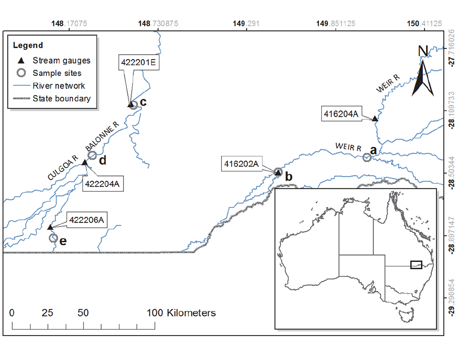
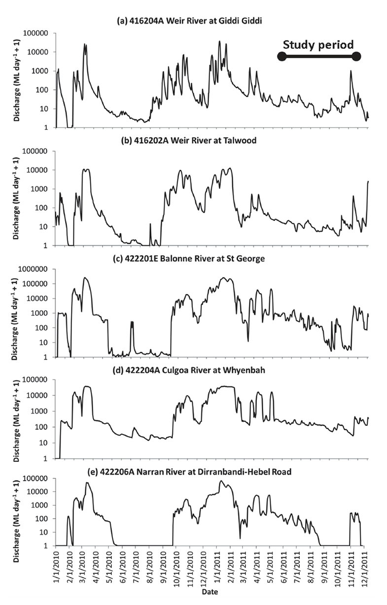
The Weir, Narran, and Balonne Rivers are collectively referred to as the Border Rivers because they straddle the Queensland/New South Wales border in eastern Australia (Fig. A1). As is common in dryland regions of the world, the river network alternates between flood and drought conditions, regularly contracting back to a series of disconnected waterholes during dry periods (Bunn et al. 2006). Prior to sampling, the region experienced significant rainfall and flooding, resulting in overbank events between December 2010 and April 2011 (Fig. A2, Marshall et al. 2012). Floodplain width varied from 270 to 11,100 m across sites, as estimated from Landsat imagery; this range was a function of bank height and position in catchment.
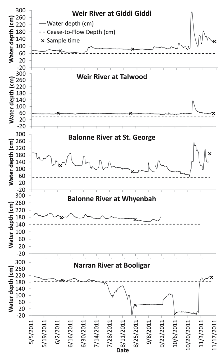
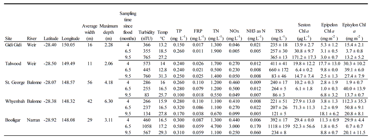
Sampling commenced approximately four months after the recession of the flood peak. However, intermittent rain events over the course of the study meant that there was flow at all sites and times except one, the exception occurring apparently due to artificial drawdown of one of the waterholes (Narran River at Booligar, Fig. A3, Marshall et al. 2012). Detailed bathymetry surveys conducted prior to biological sampling allowed calculation of cease to flow depths, and continuous depth loggers showed that cease to flow depths were not reached at any point with the one exception at Booligar (Fig. A3). During the sample period, the waterholes were shallow, narrow, turbid and productive (Table A1).
A.2 Collection of sources and consumers
Based on prior work in the region, we expected periphyton to be the dominant food source pathway for fishes (Bunn et al. 2003, Jardine et al. 2013). We therefore sampled this source extensively by collecting three replicates each of epipelon (periphyton on mud) and epixylon (periphyton on wood) at every site and time, and analyzing each as a bulk sample and after purification using colloidal silica (Hamilton et al. 2005). We ultimately used the data from the purified samples as representative of the periphyton source pathway because C/N ratios, one indicator of the relative proportion of terrestrial detritus and algal material in the sample (Jardine et al. 2014), were lower in purified samples [average difference (bulk – purified) = 4.2 for epipelon and 0.6 for epixylon].
Seston was collected by filtering subsurface water samples onto glass fibre filter papers. All other plant material was collected by hand, including submerged, conditioned leaf litter, fresh herbaceous riparian vegetation, and pasture grasses. The three categories of higher plants were analyzed as separate pooled samples within sites because they were likely to differ isotopically (due to C3 and C4 photosynthetic pathways, O’Leary 1988) and in their FA profiles.
Invertebrates were sampled using standard techniques and analysed as pooled samples of multiple individuals. Zooplankton were collected using 500 m subsurface tows just before dusk. Terrestrial invertebrates were gathered with sweep nets, and we attempted to sample two common taxa [ants (Formicidae) and grasshoppers (Orthoptera)] at each site and time. Zoobenthos was sampled with D-frame kick nets and sweep nets in the littoral zone. Samples were identified to the order or family level in the field to allow sample splitting for SIA and FAA. We also collected a sample of palaemonid prawns (Macrobrachium australiense) at each site and time because they are large-bodied and abundant and play important trophic roles as both predators and prey (Jardine et al. 2013).
Fish sampling was conducted using overnight fyke net sets and seine net drags through the littoral zone. All fish were weighed and measured on site and a subset was retained for laboratory analyses. Because we intended to measure isotopes and FA in the dominant fish species to characterize energy flow, based on prior knowledge of these systems we targeted three species with different diets and life histories that were likely to be common and abundant. These were the omnivore, invasive European carp (Cyprinus carpio) and two native species, the algivore/detritivore bony bream (Nematalosa erebi) and the predator golden perch (Macquaria ambigua) (Sternberg et al. 2008). The a priori selection of these three species proved to be appropriate because they made up an average of 85% of the biomass at different sites and times (Table A2). There were, however, other species that occasionally accounted for a significant proportion of the biomass at a particular site on a particular date (max contribution = 21%), so we added three more species on our final sampling trip to characterize their diet with isotopes and FA. These species were the native Hyrtl’s tandan Neosilurus hyrtlii and spangled perch Leiopotherapon unicolor, and the invasive goldfish Carassius auratus. Snake-necked turtles (Chelodina longicollis) that were caught occasionally in fyke nets were also sampled by removing a small biopsy from the toe.
Consistent with prior work in this basin (Forsyth et al. 2013), carp dominated the biomass of these waterholes (Table A2) with a peak yield of 109 kg from a single overnight fyke net set (249 individuals at an average mass of 436 g). Highest carp CPUE occurred on the third sampling trip at all 5 sites. To determine the overall contribution of source pathways to fish biomass using SIA, we used methods outlined in Jardine et al. (2013) and Jardine (2014). First, we calculated median contributions to the diet from each of four source pathways (plankton, periphyton, C3 plant detritus, and C4 plant detritus; see Isotope mixing models in A.4 below) for each fish species. We then multiplied the median contribution by the species’ biomass and summed the totals. This provides an estimate of the total standing biomass in the fish community that originated with a particular source (Jardine et al. 2013).
A.3 Laboratory methods for fatty acid extraction and esterification
After freeze-dried samples were immersed in chloroform overnight, a solution of methanol (1 mL), 2:1 chloroform-methanol (1 mL), and NaCl (0.8 mL; salt wash) was added and samples topped with N2. Sonication and vortexing were then employed to further break up sample tissue. Following centrifugation, the lipid layer (bottom organic layer) was collected by double pipetting - using a long Pasteur pipette inside a short one. The collected material was transferred into a pre-cleaned vial and stored on ice under N2. The mixture was washed three times with ice-cold chloroform (3 mL) repeating sonication, vortexing, centrifugation, and removal of the organic layer each time. The amount of total lipids was determined gravimetrically by weighing aliquots of lipid extracts (duplicates) on a microscale (±1 µg; Sartorius™) as a measure of the required quantity for subsequent formation of fatty acid methyl esters (FAME).
For esterification, the total lipid extracts were evaporated under N2, and toluene (1 mL) and H2SO4-methanol (2 mL; 1% v/v) were added, vortexed, and stored for 16h at 50°C (Schleichtriem et al. 2008). Subsequently, KHCO3 (2 mL; 2% v/v) and BHT (butylated hydroxytoluene, 5 mL; 0.01%) were added, shaken, and CO2 released. After centrifugation the top layer was removed. BHT (5 mL) addition, CO2 release, centrifugation and removal of the top layer were repeated and the formed FAME were dried under N2 and re-dissolved in hexane.
A.4 Isotope mixing models
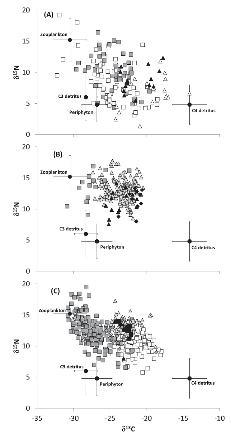
For the planktonic end-member, because of the difficulties in obtaining pure samples of phytoplankton (Hamilton et al. 2005), we used zooplankton as a proxy and assumed their diet was dominated by phytoplankton with minor contributions from other sources (Cole et al. 2011, Jardine et al. 2013). Recognizing that there is considerable temporal variation in isotope ratios of short-lived, fast turnover algal species and zooplankton (Cabana and Rasmussen 1996, Jardine et al. 2014), we used mean values and associated error for all five sites during all three sampling periods, thereby taking into account the spatial and temporal isotopic variation in source pathways. While this inflated the error around each source, the large isotopic difference among the most distal end-members (e.g., plankton and C4 detritus) allowed reasonable resolution in the mixing models (Parnell et al. 2010). The end-member values we used for all mixing model calculations were as follows: plankton δ13C = -31.3 ± 2.3‰, δ15N = 10.4 ± 3.4‰ (n = 31); periphyton δ13C = -26.8 ± 2.1‰, δ15N = 4.8 ± 2.8‰ (n = 68); C3 plant detritus δ13C = -28.3 ± 1.6‰, δ15N = 6.0 ± 3.7‰ (n = 78); C4 plant detritus δ13C = -14.1 ± 2.4‰, δ15N = 4.8 ± 3.2‰ (n = 40) (Fig. A4).
Our first approach was to examine the contribution of sources to taxonomic groups (orders for insects, families for crustaceans, species for fishes) to examine overall energy flows to the food web (Jardine et al. 2013, Jardine 2014). We did not obtain quantitative biomass data for the invertebrates, so source proportions are for commonly collected taxa rather than biomass-weighted as we calculated for fishes. We used trophic enrichment factors (TEFs) from Bunn et al. (2013) to back-calculate from the δ15N of the consumer of interest to the underlying source. This approach accounts for the number of trophic steps between the source and consumer. We used source-to-consumer TEFs for herbivorous insects (0.6 ± 1.7‰, applied to Ephemeroptera, Trichoptera, Chironomidae, Corixidae and other non-predaceous Coleoptera), predatory insects (1.8 ± 1.7‰, applied to Odonata, Dytiscidae, Notonectidae, and Gerridae), herbivorous fishes (3.9 ± 1.4‰, applied to bony bream that were grouped as small < 100mm total length and large > 100mm total length), omnivorous fishes (4.3 ± 1.5‰, applied to carp, hyrtl’s tandan, spangled perch, and goldfish) and predatory fishes (5.7 ± 1.6‰, applied to golden perch) (Bunn et al. 2013). We assumed turtles were omnivorous and chose a TEF equivalent to omnivorous fishes (4.3 ± 1.5‰), while crustaceans are predatory so we used the predatory invertebrate TEF (1.8 ± 1.7‰). For terrestrial insects and mollusks, we did not have reliable TEF data for the region, so we used a literature-derived estimate for these taxa with a common error estimate (2.5 ± 1.7‰, Vanderklift and Ponsard 2003). For all taxa, we assumed a TEF of 0‰ for δ13C (Post 2002), but incorporated an error estimate of 1.7‰. Because TEFs can influence SIAR outputs (Bond and Diamond 2011), we tested for sensitivity in a subset of taxa and found that source proportions varied little with choice of TEF.
Table A1. Environmental data for waterholes in southwestern Queensland, Australia, where food webs were sampled for SIA and FAA.
Table A2. Fish biomass (g) collected per species on three sampling trips (Trip 1 = June 2011, Trip 2 = August 2011, Trip 3 = November 2011) at five sites in the Border Rivers, Queensland (B = Narran River at Booligar, G = Weir River at Gidi Gidi, S = Balonne River at St. George, T = Weir River at Talwood, W = Balonne River at Whyenbah).
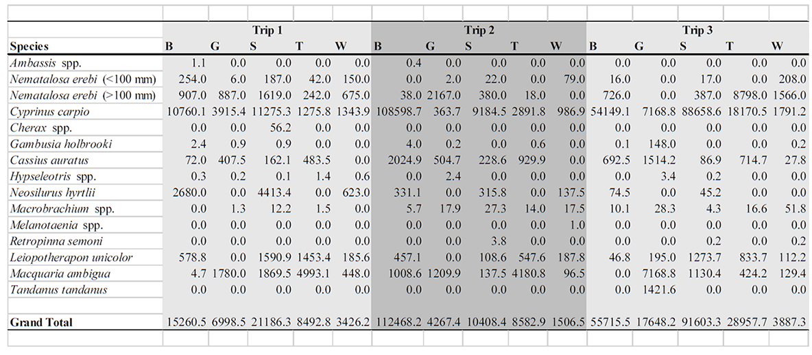
Fig. A1. Map of the study area showing the five waterholes [open circles: (a) Weir River at Gidi Gidi, (b) Weir River at Talwood, (c) Balonne River at St. George, (d) Balonne River at Whyenbah, (e) Narran River at Booligar] where food web sampling was conducted, as well as Australian Bureau of Meteorology stream gauges (solid triangles).
Fig. A2. Discharge hydrographs for the period preceding and during the study, measured at gauges in the near vicinity of the five study waterholes in the Border Rivers system, southwestern Queensland. See Fig. A1 for gauge locations.
Fig. A3. Water level during the study period at fiver waterholes in southwestern Queensland. Cease to flow depths were determined by detailed bathymetric surveys.
Fig. A4. Biplot of stable carbon (δ13C) and nitrogen (δ15N) isotopes for sources (solid circles) and (a) insects (open squares = herbivorous aquatic; shaded squares = predatory aquatic; solid triangles = terrestrial Formicidae; open triangles = terrestrial Orthoptera), (b) other animals (shaded squares = mollusks; shaded triangles = Macrobrachium australiense; solid triangles = Cherax spp.; solid diamonds = Chelodina longicollis) and (c) fishes (shaded squares = bony bream, shaded triangles = golden perch, open squares = carp, solid triangles = hyrtl’s tandan, solid squares = spangled perch, shaded diamonds = goldfish).
Literature cited
Bond, A. L., and A. W. Diamond. 2011. Recent Bayesian stable-isotope mixing models are highly sensitive to variation in discrimination factors. Ecological Applications 21:1017–1023.
Bunn, S. E., P. M. Davies, and M. Winning. 2003. Sources of organic carbon supporting the food web of an arid zone floodplain river. Freshwater Biology 48:619–635.
Bunn, S. E., M. C. Thoms, S. K. Hamilton, and S. J. Capon. 2006. Flow variability in dryland rivers: Boom, bust and the bits in between. River Research and Applications 22:179–186.
Bunn, S. E., C. Leigh, and T. D. Jardine. 2013. Diet-tissue fractionation of δ15N by consumers from streams and rivers. Limnology and Oceanography 58:765–773.
Cabana, G., and J. B. Rasmussen. 1996. Comparison of aquatic food chains using nitrogen isotopes. Proceedings of the National Academy of Sciences USA 93:10844–10847.
Cole, J. J., S. R. Carpenter, J. F. Kitchell, M. L. Pace, C. T. Solomon, and B. C. Weidel. 2011. Strong evidence for terrestrial support of zooplankton in small lakes based on stable isotopes of carbon, nitrogen, and hydrogen. Proceedings of the National Academy of Sciences USA 108:1975–1980.
Hamilton, S. K., S. J. Sippel, and S. E. Bunn. 2005. Separation of algae from detritus for stable isotope or ecological stoichiometry studies using density fractionation in colloidal silica. Limnology and Oceanography-Methods 3:149–157.
Jardine, T. D. 2014. Organic matter sources and size structuring in stream invertebrate food webs across a tropical to temperate gradient. Freshwater Biology 59:1509–1521.
Jardine, T. D., R. J. Hunt, S. J. Faggotter, D. Valdez, M. A. Burford, and S. E. Bunn. 2013. Carbon from periphyton supports fish biomass in a wet-dry tropical river. River Research and Applications 29:560–573.
Jardine, T. D., W. L. Hadwen, S. K. Hamilton, S. Hladyz, S. M. Mitrovic, K. A. Kidd, W. Y. Tsoi, M. Spears, D. P. Westhorpe, V. M. Fry, F. Sheldon, and S. E. Bunn. 2014. Understanding and overcoming baseline isotopic variability in running waters. River Research and Applications 30:155–165.
Marshall, J. C., R. J. Woods, J. S. Lobegeiger, and J. H. Fawcett. 2012. Landscape setting of the study sites: hydrology, floodplain extent, waterhole morphology and waterhole persistence. Pages 20–51 in R. J. Woods, J. S. Lobegeiger, J. H. Fawcett, and J. C. Marshall, editors. Riverine and floodplain responses to flooding in the Lower Balonne and Border Rivers – Final Report. Department of Environment and Resource Management, Queensland Government.
O’Leary, M. H. 1988. Carbon isotopes in photosynthesis. BioScience 38: 328–336.
Post, D. M. 2002. Using stable isotopes to estimate trophic position: models, methods and assumptions. Ecology 83:703–718.
Schleichtriem, C., R. J. Henderson, and D. R. Tocher. 2008. A critical assessment of different transmethylation procedures commonly employed in the fatty acid analysis of aquatic organisms. Limnology and Oceanography: Methods 6: 523–531.
Sternberg, D., S. Balcombe, J. Marshall, and J. Lobegeiger. 2008. Food resource variability in an Australian dryland river: evidence from the diet of two generalist native fish species. Marine and Freshwater Research 59:137–144.
Vanderklift, M. A., and S. Ponsard. 2003. Sources of variation in consumer-diet delta N-15 enrichment: a meta-analysis. Oecologia 136:169–182.