Ecological Archives E096-274-A1

P. S. Petraitis and S. R. Dudgeon. 2015. Variation in recruitment and the establishment of alternative community states. Ecology 96:3186–3196. http://dx.doi.org/10.1890/14-2107.1

Appendix A. Seven tables and three figures that present additional analysis and graphs supporting the results and conclusions.

Table A1. Dates and duration of when recruitment surfaces were deployed. Information based on when recruitment surfaces were in the water from 1997 to 2012. The standardizations are number per 1 sq cm per 56 days for fucoids, number per 100 sq cm per 56 days for barnacles (S. balaniodes) and number per 40 sq cm per 84 days for mussels (M. edulis). Fucoid recruits were a mixture of Ascophyllum nodosum and Fucus vesiculosus because adults of both species were present at our sites. The embryos of the two species are indistinguishable and young germlings (< 2 months of age) can be identified by the presence of apical hairs in Fucus and their lack in Ascophyllum. The recruitment tiles were specifically set out during the peak of Ascophyllum recruitment and at a time when Fucus typically does not recruit. We assume the majority of the recruits were Ascophyllum but cannot be certain.

Table A2. Deltas and AIC weights for the best-supported models of recruitment; 43 models were compared. See Appendix B for definitions of delta and weight, and Supplement 3 for data file and R scripts. Model ID column gives model identifier used in the R script.

Table A3. Permutation tests for constrained analysis of proximities. Analysis was run using capscale() function in vegan. Size, Year and Bay were included as main effects, and Site was included as random effect (i.e., included in model statement as a Condition), which structures how the permutations were done. Bay does not appear in the output because of confounding with Site. See Supplement 3 for R script and data file.

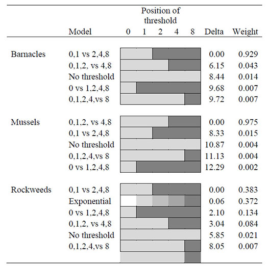
Table A4. Deltas and AIC weights for best-supported models testing the position of the threshold. For barnacles and mussels, we compared five models. Four of the models tested for breaks or thresholds between different sized clearings. The fifth model tested for no effect due to clearing size (i.e., size was not included as a factor). For fucoids, we added a sixth model in which tested for an exponential decline because Dudgeon and Petraitis (2001) reported this pattern for rockweeds. See Appendix B for definitions of delta and weight, and Supplement 3 for data file and R script.

Table A5. Corrected AICs (AICc), deltas and AIC weights for all models constructed using cusp in R. Seven different models were evaluated (Burnham and Anderson 2002); models differed in the how recruitment rates were included in the estimation of parameters. See Appendix B for definitions of delta and weight, and Supplement 4 for data file and R script. Model ID column gives model identifier used in the R code. Columns b, m, and f denote barnacle, mussel and fucoid recruitment, respectively. Note that cusp() also fits linear and logistic models; AICc’s for these models were >150 in all cases.

Table A6. Estimates and SE's for best-supported cusp model (model 6 in Table A5). Labels in “Measured variables” column match identifiers found in datasets and output of the R script for running the cusp models (see Supplement 4): w[uSB] = coefficient that is multiplier (i.e., the weighting) for understory cover by S. balanoides, w[cFV] = weighting for canopy cover by F. vesiculosus, w[uME] = weighting for understory cover by M. edulis, w[uAN] = weighting for canopy cover by A. nodosum. The solutions for Y are found by solving the equation:  (Gilmore 1981, Grasman et al. 2009).

Table A7. Mantel tests of concordance in recruitment pre and post scraping. Entries r and p are the Mantel correlation and the p value based on randomization tests. Note we also examined cross-correlations between fucoid, barnacle and mussel recruitment as shown in the pre vs. pre and post versus post entries. There were significant cross-correlations between mussels and barnacles. See Supplement 5 for data files and R scripts.

Table A8. Deltas and AIC weights for the best-supported models of the effects of scraping as a predictor. See Appendix B for definitions of delta and weight, and Supplement 6 for data file and R script. Model ID column gives model identifier used in the R code; note the best-supported models are the same for all species.

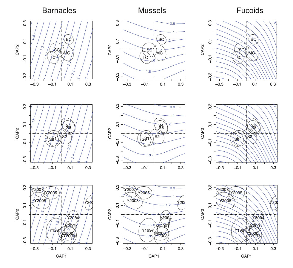
Fig. A1. Plots of CAP results with log-transformed recruitment as contour lines. The three rows of panels show centroids and 95% confidence ellipses for bays, size of clearing, and year. For bays: TC = Toothacker Cover, BC = Burnt Coat Harbor, SC = Seal Cove, and MC = Mackerel Cove. For size of clearing, S0 = uncleared control, S1= 1 m clearing, S2 = 2 m clearing, S4 = 4 m clearing, and S8 = 8 m clearing. The three columns of panels labeled Mussels, Barnacles and Fucoids show the contours defined by each taxon. The numbers on the isoclines are recruitment rates as log-transformed numbers; e.g., the line labeled 1.2 on the barnacle plots is the isocline for 14.85 barnacle recruits per 100 cm² per 56 days (log₁₀(14.85+1) = 1.2). Isoclines for fucoid plots range from 0.3 (in upper right corner of plots) to 2.1 (in lower left corner). Note all nine plots are scaled the same so the spread of centroids and confidence ellipses are directly comparable. Year that is not fully shown on the left side of the plots is 2006.

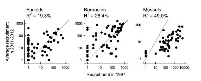
Fig. A2. Relationship between recruitment in 1997 and average recruitment in 2011–2012 for fucoids, barnacles and mussels. Axes are in logs; and zeros indicate no recruitment (i.e., log(x+1) where x=0). Solid lines are 1:1 lines.

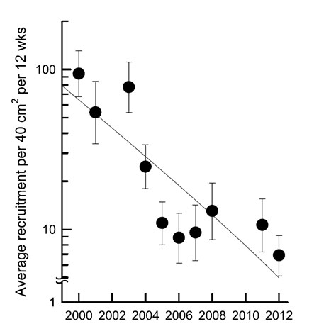
Fig.A3. Decline in mussel recruitment from 2000 to 2012. Averages and 95% CL. Line is fitted as a linear OLS regression across years for each plot using log(x+1) transformed data (n = 60 plots). We had data for 10 or 11 years for nearly all plots (average = 10.7). Regressions were done using Jmp Pro 10; meta-analyses were carried out in Excel using the inverse of mean square errors as weights. Estimates were back-transformed and reported as average percent change per year with 95% confidence limits.

Literature cited

Burnham, K. P., and D. R. Anderson. 2002. Model Selection and Multi-Model Inference: A Practical Information-Theoretic Approach. Second edition. Springer.

Dudgeon, S., and P. S. Petraitis. 2001. Scale-dependent recruitment and divergence of intertidal communities. Ecology 82:991–1006.

Gilmore, R. 1981. Catastrophe Theory for Scientists and Engineers. John Wiley and Sons, New York, New York, USA.

Grasman R.P.P.P., H.L.J. van der Maas, and E.J. Wagenmakers. 2009. Fitting the cusp catastrophe in R: A cusp package primer. Journal of Statistical Software 32:1–27.

[Back to E096-274]