Ecological Archives E096-263-A3
Howard B. Wilson, Jonathan R. Rhodes, and Hugh P. Possingham . 2015. Two additional principles for determining which species to monitor. Ecology 96:30163022. http://dx.doi.org/10.1890/14-1511.1
Appendix C. The performance of the combined principles with unequal monitoring costs.
Numerical simulations were used to investigate the efficiency of the rules when the costs of monitoring were significant as compared to the cost of taking conservation actions, and the costs of monitoring differed substantially among species. Three strategies for the allocation of monitoring resources were analysed: a random allocation of monitoring funds; allocate resources to the species which are the cheapest to monitor; and allocate monitoring funds based on our combined rules (VoM, the value of monitoring). These were all compared to an estimate of the optimal allocation of the monitoring budget. A total budget of $50M was used, 90% was allocated for conservation action ($45M), 10% for monitoring ($5M). The cost of conservation action for each species was randomly taken from a uniform distribution between $0.5M - $1.5M. The exact monitoring cost for each species was randomly taken from a uniform distribution, centered at $0.25M and steadily widened to $0 - $0.5M. As the distribution widns, the variation in monitoring cost between species increased, and the effect on the performance of the different strategies was quantified. The probability of decline for each species was a uniformly distributed random number between zero and one. Simulations used 100 species and the results were an average over 10,000 simulations.
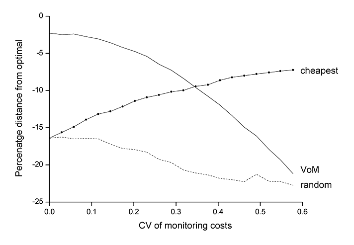
When the cost of taking conservation actions to reverse declines was much greater than the cost of monitoring to detect declines (i.e., the ratio Mi / Ci is small), then monitoring costs (whether equal or unequal between species) are not influential in determining the best species to monitor. Here this ratio was set at 0.25 (i.e., less than one but not particularly small), and we analysed how the variance in monitoring costs between species affected our results. Our combined rules were close to optimal (within 2.5%) when monitoring costs were equal (Fig. C1). It was 14% better than a random allocation of monitoring effort. As monitoring costs were increasingly different between species, then the combined rules worked progressively less optimally, but still always performed substantially better than random (figure C1). An allocation of monitoring resources solely based on monitoring the cheapest species worked progressively better as the variance in monitoring costs between species increased, and performed better than the combined rules when the coefficient of variation in the monitoring costs was greater than approximately 0.35.
Fig. C1. The performance of different monitoring strategies with increasing differentiation of monitoring costs between species. The x-axis is the coefficient of variation (CV) of the monitoring costs. The y-axis is the percentage difference in the numbers of species declining between each strategy and an estimate of the optimal distribution of monitoring resources (using the formulae in the main text). The ‘random’ strategy (dashed line) randomly chooses species to monitor until the monitoring budget is used up. The ‘cheapest’ strategy (line with symbols) monitors those species that are cheapest to monitor, in increasing order of cost, until the monitoring budget is used up (when all the species have the same monitoring cost then this is the same as the random strategy). The VoM strategy (full line) allocates monitoring based on the two combined rules.