Ecological Archives E096-257-A1
Andrew J. Allstadt, Andrew M. Liebhold, Derek M. Johnson, Robert E. Davis, and Kyle J. Haynes. 2015. Temporal variation in the synchrony of weather and its consequences for spatiotemporal population dynamics. Ecology 96:29352946. http://dx.doi.org/10.1890/14-1497.1
Appendix A. Statistical properties of the moving window correlations.
Mean and variance of synchrony estimates
Throughout our study we calculated synchrony using a 3-year moving window, the shortest window possible to calculate inter-annual correlations and shorter than the ≥15-year windows of previous studies (e.g., Ranta et al. 1998, Post and Forchhammer 2004, Bjørnstad et al. 2008). This short time window maximized temporal resolution and minimized problematic autocorrelation, but raised questions about its effectiveness. Here, we study the statistical properties of this measurement using simulated data from the population model described in the main text.
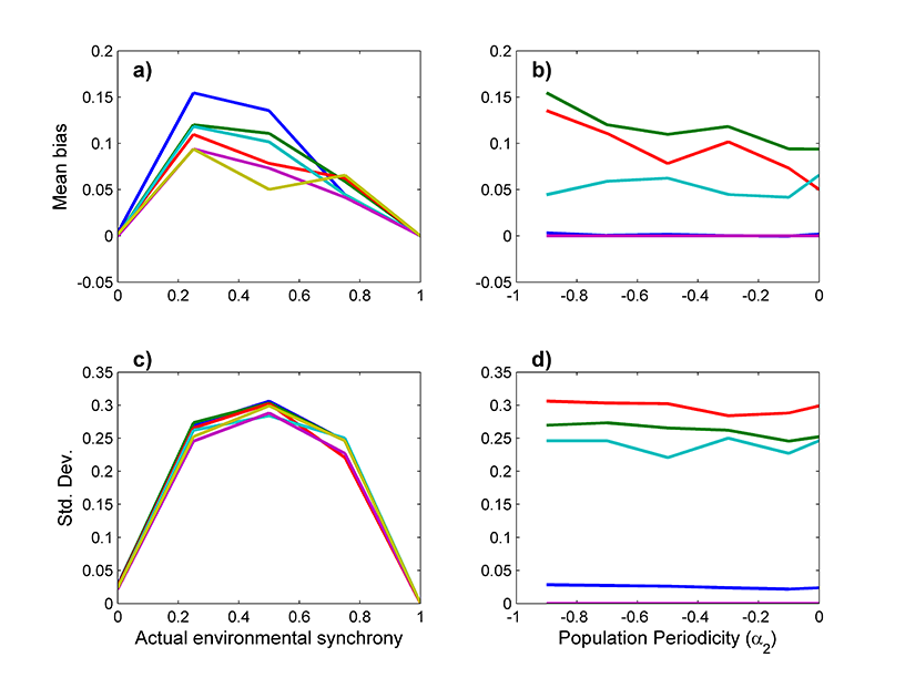
To test for bias and variability in these estimates, we ran the simulation model described in the main text with a constant level of environmental synchrony for 5000 years. We repeated this process for a variety of levels of environmental synchrony, and for various levels of periodicity in the local population dynamics. In all simulations, the classic time-invariant Moran effect holds even when SE varies through time. Overall, the 3-year window tends to overestimate the actual environmental synchrony, particularly at intermediate levels of environmental synchrony. Similarly, the standard deviation, or noisiness, of these estimates is highest for intermediate levels of environmental synchrony (Figure A1c). Much of the noisiness in these estimates at intermediate levels of environmental synchrony can be attributed to phase dependence caused by partially synchronized, system-wide population cycles (see main text and Appendix D). As demonstrated in Fig. A2 and in the simulation model results in the main text, this phase dependence does not prevent detection of relationships between environmental synchrony and population synchrony.
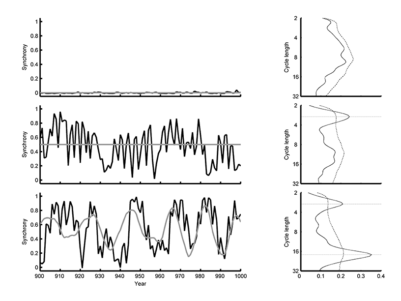
Though we minimized autocorrelation with our short time window, we were concerned that remaining serial autocorrelation could interfere with our analyses. Of particular importance would be something similar to the Slutzky-Yule effect, in which moving window averages can create spurious autocorrelation and periodicity in a time series (Royama 1992). Therefore, we considered the autoregressive properties of the 3-year moving window process using the simulation described in the main text, but with environmental synchrony set to zero. We varied the parameters governing local population dynamics as described in the main text, as well as the variance of stochasticity affecting each local population. The standard deviation of the resulting synchrony time series were >0.01 for all parameter values (Fig. A2, top row). The level of variation was more than an order of magnitude lower than that in our observed time series (e.g., Appendix C) or in our simulation model with positive, but less than perfect, synchrony (e.g., Fig. A1c). Spurious periodicity also did not affect results from simulations with constant, positive levels of environmental synchrony (Fig. A2, middle row). In this case, changes in population synchrony were dominated by the phase dependence of population synchrony on cycles in regional population density (Appendix D). Simulations with fluctuations in environmental synchrony indicated periodicity due to phase dependence, as well as variation in environmental synchrony (Fig. B2, bottom row). We concluded that any temporal variability introduced by the 3-year window would be inconsequential given the larger effect of variation in environmental synchrony and phase dependence (Appendix D).
Fig. A1. (a, b) Average bias and (c, d) standard deviation in 3-year moving window synchrony estimates for simulation model data run with a constant level of environmental synchrony. (a, c) Colors correspond to simulations where the local population dynamics had periodicity corresponding to α2 = -0.9 (blue), -0.7 (green), -0.5 (red), -0.3 (light blue), -0.1 (purple), and 0 (yellow). (b, d) Constant environmental sychrony was set to 0 (dark blue), 0.25 (green), 0.5 (red), 0.75 (light blue), and 1 (purple).
Fig. A2. The last 50 time steps of simulation (left) and the global wavelet spectra for the entire time series (right) A simulation model examples of population synchrony (blue) tracking environmental synchrony (red) in a simulation. Here, environmental synchrony was modelled as a simple sine wave, and local populations had a period length of 6 with α2 = -0.65. In the bottom row, environmental synchrony fluctuated with a mean of 0.5, cycle length of 18 years, and δ2 = -0.95. Dashed lines in the global spectra indicate cycle lengths at which periodicity is expected, for phase dependence (3 years, see Appendix D) and tracking changes in environmental synchrony (18 years).
Literature cited
Bjørnstad, O. N., A. M. Liebhold, and D. M. Johnson. 2008. Transient synchronization following invasion: revisiting Moran’s model and a case study. Population ecology 50:379–389.
Post, E., and M. C. Forchhammer. 2004. Spatial synchrony of local populations has increased in association with the recent Northern Hemisphere climate trend. Proceedings of the National Academy of Sciences of the United States of America 101:9286–9290.
Ranta, E., V. Kaitala, and P. Lundberg. 1998. Population variability in space and time: the dynamics of synchronous population fluctuations. Oikos 83:376–382
Royama, T. 1992. Analytical population dynamics. Springer.