Ecological Archives E096-241-A3
Kurt E. Anderson, Brian D. Inouye, and Nora Underwood. 2015. Can inducible resistance in plants cause herbivore aggregations? Spatial patterns in an inducible plant/herbivore model. Ecology 96:27582770. http://dx.doi.org/10.1890/14-1697.1
Appendix C. Figures showing further examples of model spatiotemporal dynamics.
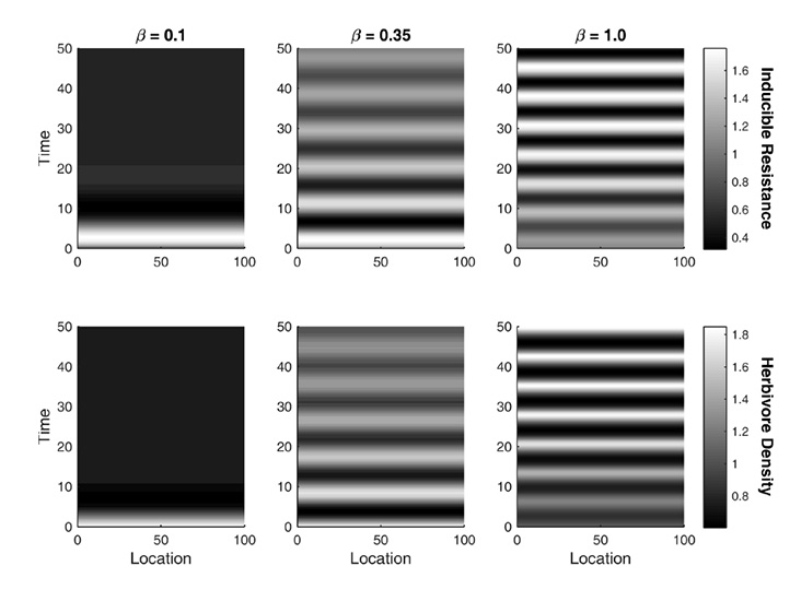
Fig. C1. Spatiotemporal dynamics exhibited by the OBEM model when the system experiences a uniform perturbation. Dynamics were obtained via numerical simulation of the full non-linear model over one hundred patches with periodic boundary conditions. Each location represents a patch. In each example, herbivores have an initial density that is 10% above the uniform steady state, while inducible resistance is at its uniform steady state. The strength of induction on mortality β is varied. When β is small, the system quickly returns to its uniform steady state. When β increases, however, the system becomes less stable; exhibiting damped and eventually sustained oscillations that are synchronized across patches. Other parameter values are τ = 2.0, χ = 30.0, D = 12.0, b = 1.0, θ = 5.0.
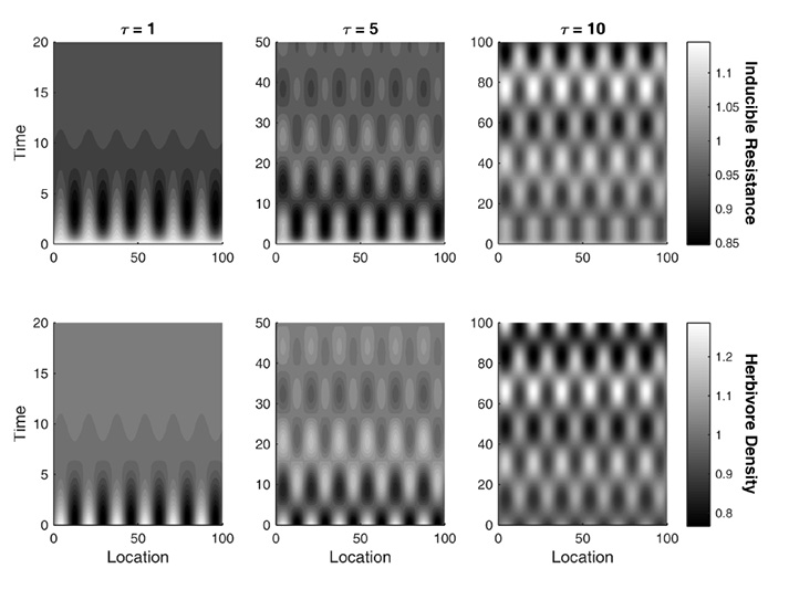
Fig. C2. Spatiotemporal dynamics exhibited by the LBME model with different time delays in the onset of induction. In these cases, the induction shape parameter θ = 1, meaning that it does not exhibit a sigmoid shape. Dynamics were obtained via numerical simulation of the full non-linear model over one hundred patches with periodic boundary conditions. Each location represents a patch. In each example, herbivores have an initial density that varies across patches as a sine wave with a spatial frequency k = 1.047, which corresponds to a spatial wavelength of ≈ 17 patches. Inducible resistance is at its uniform steady state. The scale of the time axis varies among scenarios for presentation purposes. Other parameter values are r = 0.1, β = 0.3, χ = 1.0, D = 0.1, b = 1.5.