Ecological Archives E096-233-A3

Connor R. Fitzpatrick, Anurag A. Agrawal, Nathan Basiliko, Amy P. Hastings, Marney E. Isaac, Michael Preston, and Marc T. J. Johnson. 2015. The importance of plant genotype and contemporary evolution for terrestrial ecosystem processes. Ecology 96:2632–2642. http://dx.doi.org/10.1890/14-2333.1

Appendix C. Results from linear mixed effect modeling for each ecosystem assay, best-fitting models for each ecosystem assay using a model comparison approach, and a figure illustrating the variance explained by herbivory, plant genotype, evolution, and spatial variation for each ecosystem assay.

Table C1. Effects of plant genotype, genotypic composition (GC 1 and 2), and biotic and abiotic factors on ecosystem processes. Genotypic composition of O. biennis within each plot quantifies the evolutionary divergence among plots between 2007 and 2011 using correspondence analysis (see Methods). The ecosystem processes measured include leaf decay in the field and lab, substrate induced respiration rate, N mineralization rate, and O. biennis seedlingperformance. We used a backwards stepwise elimination procedure to find the best fitting model for each ecosystem variable (see Methods), and we show results for the final model. Effects that were eliminated from the final model are shown by “-“. The significance of all effects were determined using log-likelihood ratio tests, fit to a χ² distribution with df = 1. We used restricted maximum likelihood and maximum likelihood to determine the significance of random and fixed effects, respectively. Effects that are significant at P < 0.05 are shown in bold.

Table C2. Effects of plant genotype, Euclidean distance and biotic and abiotic factors on ecosystem processes. Euclidean distance of O. biennis populations quantifies the magnitude and rate of evolution within plots between 2007 and 2011 (see Methods). The ecosystem processes measured included leaf decay in the field and lab, substrate induced respiration rate, N mineralization rate, and O. biennis seedlingperformance. We used a backwards stepwise elimination procedure to find the best fitting model for each ecosystem variable (see Methods), and we show results for the final model. Effects that were eliminated from the final model are shown by “-“. The significance of all effects were determined using log-likelihood ratio tests, fit to a χ² distribution with df = 1. We used restricted maximum likelihood and maximum likelihood to determine the significance of random and fixed effects, respectively. Effects that are significant at P < 0.05 are shown in bold.

Table C3. Best fitting models (Δ Akaike information criterion (AIC) <2), explaining variation in five ecosystem response variables. “Df” represents the model degrees of freedom, “AIC weight” represents the relative likelihood of each model compared to all others (Burnham & Anderson, 2002). “R²_m” and “R²_c” represent the marginal and conditional coefficients of determination, respectively. Factor codes include “A” abundance, “B” genotype composition 1, “C” genotype composition 2 “D” genotype, “E” herbivory treatment, and the interactions “F” abundance:GC1, “G” abundance:GC2, “H” abundance:genotype, “I” abundance:herbivory treatment, “J” GC1:treatment,  “K” GC2:treatment, “L” herbivory treatment:genotype.

Table C4. Best fitting models (Δ Akaike information criterion (AIC) <2), explaining variation in five ecosystem response variables. These models contain Euclidean distance as a measure of evolutionary change instead of genotypic composition. “Df” represents the model’s degrees of freedom, “AIC weight” represents the relative likelihood of each model compared to all others (Burnham and Anderson, 2002). “R²_m” and “R²_c” represent the marginal and conditional coefficients of determination, respectively. Factor codes include “A” abundance, “B” Euclidean distance, “C” genotype, “D”  herbivore treatment, and the interactions “E” abundance:Euclidean distance, “F” abundance:genotype, “G” abundance:herbivory treatment, “H” Euclidean distance:herbivory treatment, “I” herbivory treatment:genotype. Euclidean distance was calculated by taking the square root of the sum of squared change in each genotype frequency between 2007 and 2011.

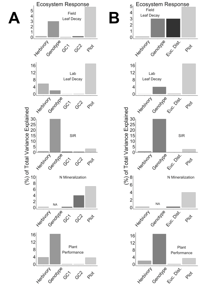
Fig. C1. The percentage of total variation explained for each ecosystem response by herbivory treatment, plant genotype, genotypic composition (A), and Euclidean distance (B), and spatial variation. Note that plant genotype explained 52% of the total variance in the soil induced respiration (SIR) assay, but we truncated the figure at 30%. We estimated the proportion of total variation explained by plant genotype, herbivory treatment, plot, and residual error using restricted maximum likelihood by fitting a model with all factors included as random effects.

[Back to E096-233]