Ecological Archives E096-233-A2
Connor R. Fitzpatrick, Anurag A. Agrawal, Nathan Basiliko, Amy P. Hastings, Marney E. Isaac, Michael Preston, and Marc T. J. Johnson. 2015. The importance of plant genotype and contemporary evolution for terrestrial ecosystem processes. Ecology 96:26322642. http://dx.doi.org/10.1890/14-2333.1
Appendix B. Study site information including plot measures of evolutionary change in Oenothera biennis populations, soil characteristics, and plant species composition, and a photograph of the ecosystem assays.
Table B1. Plot characteristics from the field experiment. We show the treatment (herbivores present vs absent), O. biennis abundance (i.e., no. individuals), genotypic composition (GC 1 and GC 2), evolutionary rate measured as Euclidean distance, and soil properties in each plot. We assessed genotypic composition by collecting tissue from 190 individual plants per plot and genotyping each sample using four microsatellite markers that provided a diagnostic identification of each of the 18 original genotypes. We then used correspondence analysis (CA) to quantify the genotypic composition (GC) of each plot based on the relative frequency of individual genotypes. Scores along the CA axes (GC1 and GC2) represent the direction of evolutionary change occurring across populations of O. biennis. Euclidean distance quantified the rate of evolutionary change within populations and it was quantified as magnitude of change in genotype between the beginning of the experiment (2007) and 2011. The insecticide treatment did not significantly alter any of the soil properties that we measured.
|
|
|
|||||||||
Treatment |
Plot |
Abundance |
GC 1 |
GC 2 |
Euclidean Distance |
Soil Moisture (%) |
pH |
Carbon (%) |
Nitrogen (%) |
C:N |
Net N Mineralization Rate (μg N/g soil/day) |
Herbivores present |
2 |
246 |
0.197 |
0.358 |
0.393 |
29.24 |
6.8 |
4.06 |
0.4 |
10.27 |
0.063 |
3 |
82 |
0.569 |
0.262 |
0.445 |
26.74 |
6.6 |
4.21 |
0.43 |
9.85 |
-0.192 |
|
5 |
482 |
0.395 |
0.362 |
0.352 |
26.64 |
6.7 |
3.95 |
0.38 |
10.46 |
0.077 |
|
7 |
508 |
0.242 |
0.33 |
0.301 |
27.49 |
6.6 |
4.36 |
0.42 |
10.47 |
0.158 |
|
8 |
524 |
0.275 |
0.316 |
0.332 |
25.75 |
6.5 |
3.37 |
0.35 |
9.75 |
0.102 |
|
10 |
226 |
0.281 |
0.401 |
0.552 |
26.48 |
6.6 |
3.37 |
0.33 |
10.14 |
-0.001 |
|
11 |
270 |
0.316 |
0.458 |
0.574 |
28.23 |
6.6 |
3.02 |
0.3 |
10.05 |
-0.027 |
|
14 |
131 |
0.391 |
0.459 |
0.565 |
26.18 |
7 |
3.14 |
0.33 |
9.51 |
0.078 |
|
27.09 |
6.7 |
3.68 |
0.37 |
10.06 |
0.032 |
||||||
Herbivores suppressed |
1 |
83 |
0.854 |
0.176 |
0.286 |
28.68 |
6.8 |
4.28 |
0.42 |
10.12 |
-0.053 |
4 |
85 |
0.356 |
0.393 |
0.355 |
28.73 |
6.7 |
3.93 |
0.4 |
9.76 |
-0.035 |
|
6 |
144 |
0.589 |
0.557 |
0.308 |
26.82 |
6.8 |
3.47 |
0.35 |
10.06 |
0.039 |
|
9 |
215 |
0.452 |
0.498 |
0.447 |
27.47 |
6.7 |
3.91 |
0.38 |
10.18 |
-0.002 |
|
12 |
819 |
0.376 |
0.453 |
0.554 |
25.66 |
6.7 |
3.11 |
0.32 |
9.83 |
-0.002 |
|
13 |
124 |
0.589 |
0.586 |
0.422 |
30.75 |
6.7 |
3.48 |
0.36 |
9.8 |
-0.127 |
|
15 |
818 |
0.505 |
0.793 |
0.538 |
29.42 |
6.7 |
3.37 |
0.35 |
9.76 |
0.176 |
|
16 |
41 |
0.495 |
0.519 |
0.561 |
29.02 |
6.7 |
3.23 |
0.34 |
9.62 |
-0.017 |
|
28.32 |
6.7 |
3.60 |
0.36 |
9.89 |
-0.002 |
||||||
Table B2. Plant species abundance data across each of our 16 plots. Abundance was recorded as the number of plants and/or proportion cover.
Solidago rugosa |
Solidago altissima |
Asclepias syriaca |
Erigeron sp. |
Silene sp. |
Solanum carolinense |
||||||
Plot |
Treatment |
Total N |
N |
% |
N |
% |
N |
N |
% |
N |
N |
1 |
I |
11 |
0 |
0.1 |
0 |
0 |
14 |
13 |
0 |
2 |
15 |
2 |
C |
13 |
0 |
0 |
0 |
0.01 |
14 |
334 |
0.44 |
2 |
0 |
3 |
C |
11 |
0 |
0 |
1 |
0 |
0 |
42 |
0 |
0 |
2 |
4 |
I |
12 |
0 |
0 |
0 |
0.33 |
0 |
12 |
0 |
4 |
17 |
5 |
C |
12 |
3 |
0.01 |
2 |
0.01 |
0 |
167 |
0.28 |
0 |
10 |
6 |
I |
10 |
0 |
0 |
0 |
0.125 |
2 |
6 |
0 |
9 |
35 |
7 |
C |
10 |
0 |
0 |
0 |
0.67 |
0 |
9 |
0 |
3 |
1 |
8 |
C |
12 |
0 |
0.01 |
0 |
0.037 |
0 |
5 |
0 |
0 |
5 |
9 |
I |
11 |
0 |
0 |
0 |
0.01 |
0 |
9 |
0 |
0 |
16 |
10 |
C |
13 |
0 |
0 |
0 |
0.17 |
0 |
26 |
0 |
2 |
7 |
11 |
C |
16 |
0 |
0.02 |
0 |
0.074 |
4 |
15 |
0 |
0 |
6 |
12 |
I |
11 |
0 |
0 |
0 |
0.11 |
5 |
12 |
0 |
0 |
21 |
13 |
I |
13 |
0 |
0.01 |
0 |
0.056 |
16 |
0 |
0 |
0 |
25 |
14 |
C |
19 |
0 |
0.01 |
0 |
0 |
22 |
5 |
0 |
1 |
15 |
15 |
I |
20 |
0 |
0.125 |
0 |
0 |
22 |
1 |
0 |
1 |
19 |
16 |
I |
18 |
0 |
0.01 |
0 |
0.074 |
26 |
0 |
0 |
0 |
34 |
Rhus sp. |
Galium sp. |
Ambrosia sp. |
Arctium minus |
Bellis sp. |
Vicia sp. |
Lathyrus sp. |
Prunus serotia |
||||
Plot |
Treatment |
N |
% |
N |
N |
% |
N |
% |
N |
N |
% |
1 |
I |
3 |
0.1 |
0.17 |
4 |
0 |
1 |
0 |
1 |
0 |
0 |
2 |
C |
0 |
0 |
0.01 |
2 |
0.05 |
0 |
0 |
0 |
0 |
0 |
3 |
C |
0 |
0 |
0 |
1 |
0.01 |
0 |
0.56 |
0 |
2 |
0 |
4 |
I |
0 |
0 |
0.11 |
1 |
0 |
0 |
0 |
0 |
0 |
0 |
5 |
C |
0 |
0 |
0 |
4 |
0.01 |
0 |
0 |
0 |
0 |
0 |
6 |
I |
0 |
0 |
0 |
1 |
0 |
1 |
0 |
0 |
0 |
0 |
7 |
C |
0 |
0 |
0 |
2 |
0 |
0 |
0 |
0 |
0 |
0 |
8 |
C |
0 |
0 |
0.037 |
0 |
0.037 |
0 |
0 |
0 |
0 |
0 |
9 |
I |
0 |
0 |
0 |
2 |
0 |
0 |
0 |
0 |
0 |
0 |
10 |
C |
0 |
0 |
0.037 |
2 |
0.01 |
0 |
0 |
0 |
0 |
0 |
11 |
C |
0 |
0 |
0.056 |
3 |
0.037 |
0 |
0 |
0 |
0 |
0 |
12 |
I |
0 |
0.1 |
0 |
6 |
0 |
0 |
0 |
0 |
0 |
0 |
13 |
I |
0 |
0 |
0 |
4 |
0.22 |
0 |
0 |
0 |
0 |
0 |
14 |
C |
0 |
0 |
0.02 |
6 |
0 |
1 |
0 |
0 |
0 |
0 |
15 |
I |
0 |
0 |
0 |
5 |
0 |
1 |
0 |
0 |
1 |
0.056 |
16 |
I |
0 |
0 |
0 |
2 |
0.01 |
0 |
0 |
0 |
0 |
0.02 |
Table B2 cont'd.
Phytolacca sp. |
Morus sp. |
Rosa sp. |
Berberis sp. |
Cirsium arvense |
Fragaria sp. |
Clematis-like plant |
Daucus sp. |
|||||
Plot |
Treatment |
N |
% |
N |
% |
% |
N |
% |
N |
% |
N |
N |
1 |
I |
0 |
0 |
0 |
0 |
0 |
0 |
0 |
0 |
0.05 |
0 |
0 |
2 |
C |
0 |
0 |
1 |
0.11 |
0 |
0 |
0 |
2 |
0 |
0 |
0 |
3 |
C |
0 |
0 |
1 |
0.0625 |
0 |
0 |
0 |
2 |
0 |
0 |
0 |
4 |
I |
0 |
0 |
2 |
0.03 |
0.08 |
2 |
0.01 |
1 |
0 |
0 |
0 |
5 |
C |
0 |
0 |
0 |
0 |
0.01 |
1 |
0 |
5 |
0 |
0 |
0 |
6 |
I |
0 |
0 |
0 |
0 |
0 |
1 |
0.02 |
0 |
0 |
0 |
0 |
7 |
C |
0 |
0 |
0 |
0 |
0 |
0 |
0 |
0 |
0.03 |
0 |
0 |
8 |
C |
0 |
0 |
0 |
0 |
0.01 |
0 |
0 |
0 |
0 |
0.074 |
0 |
9 |
I |
1 |
0.02 |
0 |
0 |
0 |
3 |
0.01 |
2 |
0 |
0 |
0 |
10 |
C |
0 |
0 |
0 |
0.125 |
0.028 |
0 |
0 |
3 |
0 |
0 |
0 |
11 |
C |
0 |
0 |
0 |
0 |
0.037 |
0 |
0 |
5 |
0 |
0 |
0 |
12 |
I |
0 |
0 |
0 |
0 |
0 |
0 |
0 |
4 |
0 |
0 |
1 |
13 |
I |
0 |
0 |
0 |
0 |
0 |
0 |
0 |
2 |
0.33 |
0 |
0 |
14 |
C |
0 |
0 |
0 |
0 |
0 |
0 |
0 |
4 |
0.01 |
0 |
0 |
15 |
I |
0 |
0 |
0 |
0 |
0 |
1 |
0 |
4 |
0 |
0 |
1 |
16 |
I |
0 |
0 |
0 |
0 |
0 |
0 |
0 |
1 |
0.33 |
0 |
29 |
|
Chenopodium sp. |
Arctium minus |
woody vine |
Mint sp. |
Phalaris sp. |
Vitis sp. |
Linaria vulgaris |
Plantago sp. |
||||
Plot |
Treatment |
N |
N |
% |
N |
N |
N |
% |
N |
% |
% |
% |
1 |
I |
0 |
0 |
0 |
0 |
0 |
0 |
0 |
0 |
0 |
0 |
0 |
2 |
C |
0 |
0 |
0 |
1 |
3 |
7 |
0.0625 |
0 |
0 |
0 |
0 |
3 |
C |
0 |
0 |
0 |
0 |
0 |
1 |
0 |
1 |
0.01 |
0 |
0 |
4 |
I |
0 |
0 |
0 |
0 |
0 |
1 |
0 |
0 |
0.01 |
0.01 |
0 |
5 |
C |
0 |
1 |
0 |
0 |
0 |
0 |
0 |
0 |
0 |
0 |
0.01 |
6 |
I |
1 |
0 |
0 |
0 |
0 |
0 |
0 |
0 |
0.028 |
0 |
0 |
7 |
C |
1 |
0 |
0 |
0 |
0 |
0 |
0 |
0 |
0.01 |
0.01 |
0 |
8 |
C |
0 |
9 |
0.333 |
0 |
0 |
2.5 |
0.01 |
0 |
0 |
0 |
0 |
9 |
I |
0 |
2 |
0.056 |
0 |
1 |
0 |
0 |
1 |
0.01 |
0 |
0 |
10 |
C |
0 |
3 |
0 |
0 |
0 |
0 |
0 |
0 |
0 |
0 |
0 |
11 |
C |
0 |
2 |
0 |
0 |
0 |
0 |
0 |
0 |
0.01 |
0 |
0 |
12 |
I |
0 |
0 |
0 |
0 |
0 |
3 |
0.02 |
0 |
0.01 |
0 |
0 |
13 |
I |
0 |
6 |
0.11 |
0 |
0 |
5 |
0 |
0 |
0.01 |
0 |
0.01 |
14 |
C |
0 |
0 |
0 |
0 |
6 |
1 |
0 |
0 |
0 |
0 |
0 |
15 |
I |
0 |
0 |
0 |
0 |
0 |
1 |
0 |
0 |
0 |
0 |
0.02 |
16 |
I |
0 |
1 |
0 |
0 |
5 |
0 |
0 |
1 |
0.01 |
0 |
0.02 |
Table B2 cont'd.
Poa sp. |
Rhamnus sp. |
Oxalis sp. |
Symphyotrichum sp. |
Hesperis sp. |
Solanum dulcamara |
Symphyotrichum novae-angliae |
|||||
Plot |
Treatment |
% |
% |
% |
N |
% |
N |
% |
N |
N |
% |
1 |
I |
0 |
0 |
0 |
0 |
0 |
0 |
0 |
0 |
0 |
0 |
2 |
C |
0 |
0 |
0 |
0 |
0 |
0 |
0 |
0 |
0 |
0 |
3 |
C |
0 |
0 |
0 |
0 |
0 |
0 |
0 |
0 |
0 |
0 |
4 |
I |
0 |
0 |
0 |
0 |
0 |
0 |
0 |
0 |
0 |
0 |
5 |
C |
0.17 |
1 |
0 |
0 |
0 |
0 |
0 |
0 |
0 |
0 |
6 |
I |
0 |
0 |
0 |
0 |
0 |
0 |
0 |
0 |
0 |
0 |
7 |
C |
0 |
0 |
0.028 |
0 |
0 |
0 |
0 |
0 |
0 |
0 |
8 |
C |
0.01 |
0 |
0 |
0 |
0.074 |
0 |
0 |
0 |
0 |
0 |
9 |
I |
0.01 |
0 |
0 |
0 |
0 |
0 |
0 |
0 |
0 |
0 |
10 |
C |
0.01 |
0 |
0.037 |
0 |
0.028 |
0 |
0 |
0 |
0 |
0 |
11 |
C |
0.01 |
0 |
0.037 |
0 |
0.02 |
1 |
0.01 |
0 |
0 |
0 |
12 |
I |
0 |
0 |
0 |
0 |
0 |
0 |
0 |
1 |
0 |
0 |
13 |
I |
0 |
0 |
0.02 |
0 |
0 |
0 |
0 |
0 |
4 |
0.02 |
14 |
C |
0 |
0 |
0.037 |
0 |
0.01 |
0 |
0 |
0 |
1 |
0 |
15 |
I |
0.028 |
0 |
0.01 |
2 |
0.015 |
0 |
0 |
0 |
5 |
0 |
16 |
I |
0 |
0 |
0.01 |
0 |
0 |
0 |
0 |
0 |
0 |
0 |
Clematis sp. |
Rumex crispus |
Viburnum dentatum |
Artemisia sp. |
Ranunculus sp. |
Lonicera sp. |
Setaria sp. |
Rubus sp. |
||||
Plot |
Treatment |
N |
N |
N |
N |
N |
N |
% |
N |
% |
|
1 |
I |
0 |
0 |
0 |
0 |
0 |
0 |
0 |
0 |
0 |
|
2 |
C |
0 |
0 |
0 |
0 |
0 |
0 |
0 |
0 |
0 |
|
3 |
C |
0 |
0 |
0 |
0 |
0 |
0 |
0 |
0 |
0 |
|
4 |
I |
0 |
0 |
0 |
0 |
0 |
0 |
0 |
0 |
0 |
|
5 |
C |
0 |
0 |
0 |
0 |
0 |
0 |
0 |
0 |
0 |
|
6 |
I |
0 |
0 |
0 |
0 |
0 |
0 |
0 |
0 |
0 |
|
7 |
C |
0 |
0 |
0 |
0 |
0 |
0 |
0 |
0 |
0 |
|
8 |
C |
0 |
0 |
0 |
0 |
0 |
0 |
0 |
0 |
0 |
|
9 |
I |
0 |
0 |
0 |
0 |
0 |
0 |
0 |
0 |
0 |
|
10 |
C |
0 |
0 |
0 |
0 |
0 |
0 |
0 |
0 |
0 |
|
11 |
C |
0 |
0 |
0 |
0 |
0 |
0 |
0 |
0 |
0 |
|
12 |
I |
0 |
0 |
0 |
0 |
0 |
0 |
0 |
0 |
0 |
|
13 |
I |
0 |
0 |
0 |
0 |
0 |
0 |
0 |
0 |
0 |
|
14 |
C |
2 |
1 |
1 |
1 |
0 |
0 |
0 |
0 |
0 |
|
15 |
I |
0 |
0 |
0 |
0 |
1 |
2 |
0 |
1 |
0 |
|
16 |
I |
0 |
0 |
0 |
0 |
1 |
1 |
0.028 |
3 |
0.01 |
|
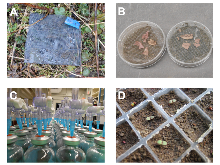
Fig. B1. Photographs showing methods used to estimate ecosystem processes and feedbacks onto plant fitness. (A) Field leaf decay - a standard amount of leaf litter from each O. biennis genotype was placed in a bag in each plot and collected at three intervals. (B) Lab leaf decay - a standard amount of leaf litter from each genotype was placed on soil taken from each plot and weighed after 60 days. (C) Substrate induced respiration - rates of CO2 respiration were measured from soil taken from each plot and placed in vials under the addition of genotype-specific litter leachate. (D) Seedling performance - seeds from each genotype planted in soil taken from each plot; biomass of seedlings was measured 7 days post-germination. Photo credit: C. Fitzpatrick.