Ecological Archives E096-194-A5
A. Coulon, J. Aben, S. C. F. Palmer, V. M. Stevens, T. Callens, D. Strubbe, L. Lens, E. Matthysen, M. Baguette, and J. M. J. Tavis. 2015. A stochastic movement simulator improves estimates of landscape connectivity. Ecology 96:22032213. http://dx.doi.org/10.1890/14-1690.1
Appendix E. Map-based comparison between methods for the natterjack toad.
It may be surmised that a visual comparison of summary maps produced by the four methods compared in this paper would be informative in terms of identifying regions of the landscape which are important for movement. In certain landscapes, and for certain classes of organism, that may well be true, but it is far from universally so, as the case study of the natterjack toad (Epidalea calamita) illustrates.
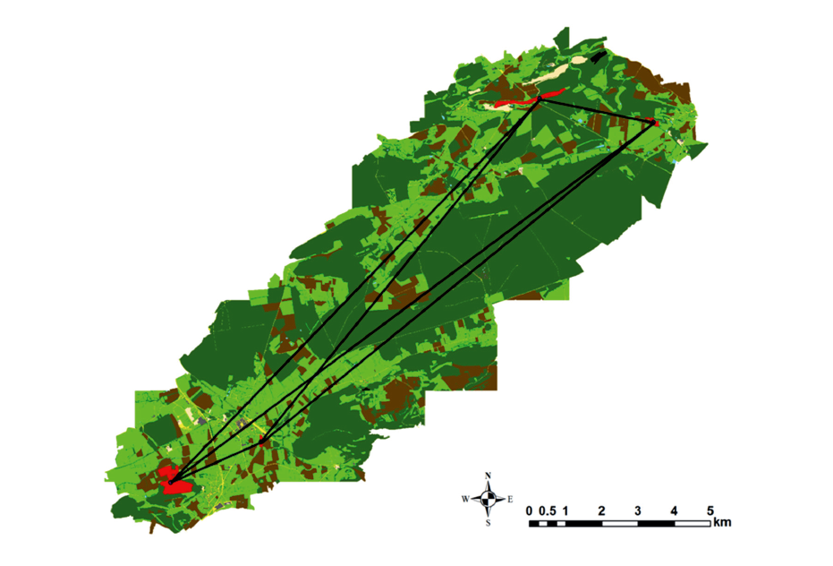
Comparison between the Euclidean distance and least cost path (LCP) connectivity estimates is straightforward, as both can be depicted as linear paths between all pairs of breeding sites (Figures E1 and E2 respectively). Whereas the straight-line Euclidean paths pass through high cost (low preference) urban areas (gray) in the SW part of the landscape, LCPs avoid such habitat, and also tend to favor woodland (dark green), the most preferred habitat. Nevertheless, the deviations of the LCP from the straight-line routes are quite limited, and thus as estimators of connectivity, the two methods differ little. Moreover, it is not clear that any particular parts of the landscape are likely to be of particularly high importance for connectivity.
In contrast, both the Circuitscape and SMS methods produce a far more diffuse picture of connectivity through the inter-site matrix (Figs. E3 and E4, respectively). They differ slightly in their finer detail, but both clearly show regions of greater ‘use’ (darker orange shades) around the pairs of sites in the NE and SW ends of the study area, and both show avoidance of the urban areas between the two SW sites (small pale yellow regions).
Why then does SMS, provided that its parameters are set to optimum values (as used for Fig. E4), substantially out-perform the other three methods in terms of its correlation with a genetic estimator of inter-site connectivity? The key lies in the central region of the landscape, where typically fewer than around 50 SMS paths out of a potential total of 40000 passed through. SMS works well in this case, because it predicts very poor connectivity (but not quite none) between the NE sites and the SW sites. In effect, the distance (over 10km) between the two pairs of sites is a substantial barrier to juvenile toads, which start their dispersal phase at only a few centimeters in size, and spend many months (possibly more than one year) moving through the landscape before potentially recruiting to a new breeding site. Only if the toads have roughly the right degree of auto-correlation in the route they take will they stand any chance in dispersing successfully over a distance in excess of 10 km. The Euclidean distance and LCP methods fail to account for this important feature of the toads dispersal ecology, as they predict connectivity respectively exactly and roughly in proportion to the distances between sites. In theory, Circuitscape should offer some advantage, over those two methods, but in this particular case, it is presumably because the range of cost values, reflecting relative habitat preferences, is quite limited (a factor of only ~1.6, excluding the relative rare urban areas), that no clear routes of low resistance, and hence high current flow, emerge. Circuitscape may be expected to perform better where there are more clearly defined movement corridors and/or barriers in the landscape, but when that is not so, SMS, by more closely mimicking in broad terms the dispersal behavior of the species at only limited extra cost in terms of additional parameters, may well prove consistently to provide the most accurate estimates of functional connectivity.
Fig. E1. Euclidean paths (black lines) between the centroids of the four breeding sites (red polygons). Cost values reflecting the relative preferences of the habitats in the inter-site matrix are as shown in Appendix B.
Fig. E2. Least cost paths (black lines) between the centroids of the four breeding sites (red polygons). Cost values reflecting the relative preferences of the habitats in the inter-site matrix are as shown in Appendix B.
Fig. E3. Current map produced by Circuitscape, showing the cumulative relative current (on a logarithmic scale) flowing through the landscape between all possible pairs of breeding sites (black polygons, where current > 1.0).
Fig. E4. Path density map produced by SMS, showing the total number of times a cell was visited (excluding multiple visits by a single individual) when 10000 SMS paths were generated from each of 4 sites (black polygons) using the preference cost layer at 3-m grain size and the SMS parameters PR = 30 m, DP = 10.0.