Ecological Archives E096-192-A5
María C. Rodríguez-Rodríguez, Pedro Jordano, and Alfredo Valido. 2015. Hotspots of damage by anatgonists shape the spatial structure of plantpollinator interactions. Ecology 96:21812191. http://dx.doi.org/10.1890/14-2467.1
Appendix E. Detailed description of spatial point pattern analyses, plus additional results from univariate and bivariate analyses of plant–animal interaction strengths and plant characteristics.
Methods
Plant spatial distribution
We characterized plant spatial distribution with the O-ring statistic O(r)as summary statistic (Wiegand and Moloney 2004, 2014). This statistic estimates the expected density of points at distance r from the typical point of the pattern. It is estimated as O(r) = λg(r), where λ is the intensity of points in the pattern, and g(r) the pair-correlation function (Wiegand and Moloney 2004). We used the estimator with edge correction, so the number of points in an incomplete circle was divided by the proportion of the area of the circle that lies within the study region. The empirical values for the statistic were compared with the theoretical values from the chosen null model, the Heterogeneous Poisson Process (HPP). We chose this null model because plants were not distributed within the patches with a constant intensity λ (first-order heterogeneity) due to the presence of gaps at the edges of the rectangular patches (Fig. E1). The presence of rocky outcrops and plant individuals of different species to Isoplexis canariensis (L.) J. W. Loudon (Plantaginaceae) caused these gaps. In the HPP model, the constant λ of the homogeneous Poisson process is replaced by a function λ (x, y), but the occurrence of any point remains independent of that of any other. In our case, the intensity function was estimated with a non-parametric method using the Box Kernel function and circular moving windows of radius = 300 cm (Wiegand and Moloney 2014).
Mark correlation functions
Mark correlation functions are summary statistics adapted for quantitatively marked patterns, where a spatial point pattern (e.g., individual plants of a given species) carries a quantitative mark (e.g., plant reproductive success). The rationale behind these functions is simple: they give the mean values of a test function calculated from the marks of all plant pairs i and j that are separated by distance r (Illian et al. 2008). The estimate of the mean value is then repeated for different r distances. Therefore, it is necessary to choose an appropriate test function that characterizes the relationship between the marks mi and mj of plants i and j. In our case, we applied two types of test functions depending on whether the marks belonged to the same or different variables.
When we analyzed the spatial relationship among marks from the same variable, we used the Schlather’s Index Im1m1(r)(Schlather et al. 2004, Wiegand and Moloney 2014). In this case, the point pattern is univariate quantitatively marked because each plant has only one mark attached. The statistic Im1m1(r)looks at pairs of plants separated by distance r and compares the marks m1 from plant i and m1 from plant j for each plant pair with the actual mean mark resulting from all pairs of plants separated by distance r. A value of Im1m1(r)~ 0 would indicate there is absence of spatial correlation among the marks. In contrast, a value of Im1m1(r)> 0 would indicate mutual stimulation, that is, plants are more similar in their mark values than expected by chance. Conversely, a value of Im1m1(r)< 0 would indicate mutual inhibition.
When marks belonged to two different variables, we used the Schlather’s Index Im1m2(r)(Schlather et al. 2004, Wiegand and Moloney 2014). The point pattern is bivariate quantitatively marked because each plant carries two marks instead of one. This approximation let us to explore if two joint properties (i.e., quantitative variables) of plants were spatially associated. Specifically, the statistic Im1m2(r)tests if the mark m1 at plant i (focal plant) and the mark m2 at plant j separated by distance r tend to be relatively similar or dissimilar compared to those of plant pairs taken at random. Again, a value of Im1m2(r)~ 0 would indicate there is absence of spatial autocorrelation among the marks m1 and m2, but in this case the mark correlation function involves marks from different variables. In contrast, a value of Im1m2(r)> 0 would indicate mutual stimulation, and a value of Im1m2(r)< 0 would indicate mutual inhibition.
In both cases, we normalized the mark correlation function with the mark variance to make it independent of the distribution and values of the marks (Wiegand and Moloney 2014). In the univariate pattern, the normalization factor coincided with the variance of the variable σ, whereas in the bivariate pattern it represented the covariance of the marks σ12 that belong to different variables. The summary statistics were first estimated separately for each patch. Then, we combined them into a single mean-weighted spatial statistic because we were interested in the broad biological pattern rather than on the potential variability among replicate patches. The formulas used to combine mark-correlation functions are detailed in Wiegand and Moloney (2014). At the end, the empirical summary statistics were compared to those arising from the null model of independent marking, which shuffles the marks independently and randomly among all plant locations (Wiegand and Moloney 2014).
Technical settings
Non-cumulative second-order statistics are based on the distance between all pairs of plants of a point spatial pattern, and they count the number of points in an annulus of radius r and width dr located at distance r from a focal plant, with r taking a range of scales. The advantage of these statistics is that the result at smaller scales does not bias the result at higher scales (Wiegand and Moloney 2004, 2014). In our case, we took into account that r < 1/2 length of the shortest side of the study patch (patch 1, max r = 500 cm), and estimated the summary statistics at distance bins of 10 cm and ring width of dr = 110 cm. The bin value indicates the interval of distance at which the statistic is calculated from the focal point. We selected the value of ring width to assure a minimum of 30 plant pairs per distance class. Note that we obtained similar results in all spatial analyses using a range of dr = 60–110 cm.
Goodness-of-Fit test
Independently of the spatial analysis, we compared the empirical values of the summary statistics to simulation envelopes arising from the corresponding null model. To create the envelopes, we used at every distance r the 25th highest and 25th lowest results for the chosen statistic (O-ring or Schlather’s Index), calculated from 999 Monte Carlo simulations (P = 0.05). The observed pattern is considered different to the simulated process if the results lie outside the envelope at any distance r. However, we cannot interpret the simulation envelopes as confidence intervals because we tested the null hypothesis at several distances simultaneously, and this approach greatly underestimates the type I error rate. As a complement to analyses based on simulation envelopes, we used a Goodness-of-Fit test (GoF). The GoF collapses the scale-dependent information contained in the test statistics into a single index ui (Loosmore and Ford 2006). This index represents the total squared deviation between the observed summary statistic and the theoretical statistic under the null model across the distance interval analyzed (0–500 cm). The ui was calculated for the observed data (i = 0) and for the simulated data (i = 1 . . .999) and the rank of u0 among all ui was determined. If the rank of u0 was > 950, there was a significant departure from the null model with α = 0.05.
Results
Spatial representation of plants, plant–animal interaction strengths and associated plant reproductive outcomes.
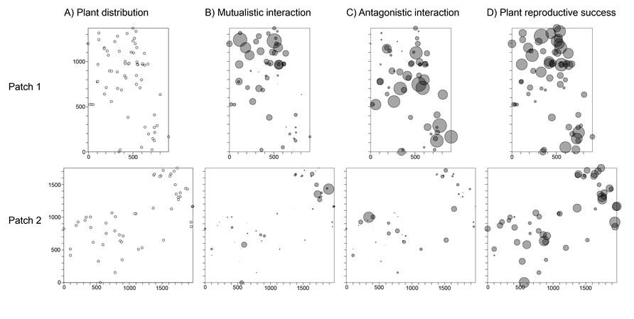
Fig. E1. (A) Spatial locations of individual Isoplexis canariensis adult plants in patch 1 (n = 67) and patch 2 (n = 52), along with their interaction strengths with mutualists (B) and antagonists (C), and associated plant reproductive success (PRS) (D). In (B–D), the circle size indicates the relative values in comparison to the largest value (mark) in the respective patch. This largest value was scaled to have a physical size of 80 units (spatstat package in R; Baddeley and Turner 2005). Patch dimensions are in cm.
Spatial analysis of plant–animal interaction strengths per animal guild
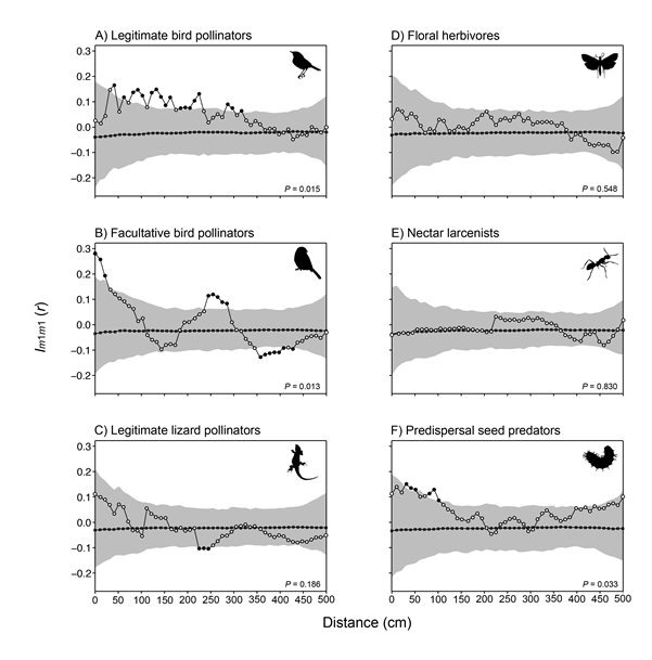
When analyzed per mutualistic guild, we found that the interaction strengths with birds were spatially structured (Fig. E2A–B), but not that with lizards (i.e., Gallotia galloti; rank = 815, P = 0.186) (Fig. E2C). In the interaction with legitimate bird pollinators (i.e., Phylloscopus canariensis, rank = 986, P = 0.015), plants were positively correlated at 40–310 cm (P < 0.05, Fig. E2A). In the case of facultative bird pollinators (i.e., Cyanistes teneriffae, rank = 988, P = 0.013), plants were positively correlated in their interaction strength at 0–20 cm and 240–280 cm, but negatively correlated at further distances 350–420 cm (P < 0.05, Fig. E2B).
A closer look to each antagonistic guild revealed the absence of spatial signal in the interaction strength with floral herbivores (rank = 453, P = 0.548; Fig. E2D) and nectar larcenists (rank = 171, P = 0.830; Fig. E2E). However, the interaction with predispersal seed predators was weakly structured (rank = 968, P = 0.033), with plants positively correlated in their interaction strength at 30–100 cm (P < 0.05; Fig. E2F).
Fig. E2. Univariate mark correlation analysis using Schlather’s Index Im1m1(r) of the interaction strength between Isoplexis canariensis plants and their mutualists: legitimate bird pollinators(A), facultative bird pollinators (B), and legitimate lizard pollinators (C); and between plants and their antagonists: floral herbivores (D), nectar larcenists (E) and predispersal seed predators (F). Dots, mean-weighted summary statistic of the data; black squares, expectation under the null model; and gray shading, simulation envelopes marking the 25th lowest and highest values taken from 999 simulations of the null model. Black dots indicate statistical difference from the null model (P < 0.05), and P values indicate statistical significance of Goodness-of-Fit (GoF) test. See Appendix A for the taxonomic composition of animal guilds.
Spatial analysis of plant characteristics, and their association with plant–animal interaction strengths.
Average plant height was 87.1 ± 38.6 cm (range = 26.5–220).Individuals had generally several inflorescences (3.8 ± 4.3 inflorescences, range = 1–25), with plants producing tens of floral pedicels (101.7 ± 122.8 pedicels, range = 8–828). When considering floral resources, I. canariensis plants had a nectar production of 20.4 ± 5.9 μL/24h/flower (range = 3.7–39.2), with 29.6 ± 6.2% of sugar concentration (range = 17.3–50.2).
Results from the univariate mark-correlation analyses of plant characteristics revealed that nearby plants were more similar in height than randomly expected (rank = 1000, P = 0.001), concretely at 0–350 cm (P < 0.05; Fig. E3A). Relative to floral resources, we did not detect a significant spatial structure in nectar production (rank = 800, P = 0.201; Fig. E3D), but we did in sugar concentration (rank = 1000, P = 0.001; Fig. E3G). Concretely, plants separated by 0–260 cm were more similar in their sugar concentration than randomly expected (P < 0.05).
In relation to the bivariate mark-correlation analyses, we detected that the mutualistic interaction strength was spatially associated with plant height (rank = 1000, P = 0.001), showing a positive correlation at r > 60 cm (Fig. E3B). The antagonistic interaction strength was also spatially associated with plant height (rank = 999, P = 0.002, Fig. E3C), and nectar production (rank = 960, P = 0.041, Fig. E3F). In the spatial association between the antagonistic interaction and plant height, we found a negative correlation at 90–340 cm (P < 0.05). In the spatial association with nectar production, we found a positive correlation at 110–260 cm, and a negative correlation at 350-380 cm (P < 0.05). The rest of spatial associations between animal interaction strengths and plant characteristics were not significant (P > 0.05 for all GoF tests).
Fig. E3. Spatial analysis of plant characteristics and their association with plant–animal interaction strengths. Univariate mark correlation analysis using Schlather’s Index Im1m1(r) of plant characteristics: plant height (A), floral nectar production (D), and nectar sugar concentration (G). Bivariate mark correlation analysis using Schlather’s Index Im1m2(r) between plant-animal interaction strengths and plant height (B–C), nectar production (E–F), and sugar concentration (H–I). Symbol interpretation is given in the legend to Fig. E2.
Literature cited
Baddeley, A., and R. Turner. 2005. spatstat: an R package for analyzing spatial point patterns. Journal of Statistical Software 12:1–42.
Illian, J.B., A. Penttinen, H. Stoyan, and D. Stoyan. 2008. Statistical analysis and modelling of spatial point patterns. John Wiley & Sons, Chichester, England.
Loosmore, N. B., and E. D. Ford. 2006. Statistical inference using the G or K point pattern spatial statistics. Ecology 87:1925–1931.
Schlather, M., P. Ribeiro, and P. Diggle. 2004. Detecting dependence between marks and locations of marked point processes. Journal of the Royal Statistical Society. Series B (Statistical Methodology) 66:79–93.
Wiegand, T., and K. A. Moloney. 2004. Rings, circles, and null-models for point pattern analysis in ecology. Oikos 104:209–229.
Wiegand, T., and K. A. Moloney. 2014. Handbook of spatial point-pattern analysis in Ecology. Chapman and Hall/CRC press, Boca Raton, Florida, USA.