Ecological Archives E096-164-A1

Ruwan Punchi-Manage, Thorsten Wiegand, Kerstin Wiegand, Stephan Getzin, Andreas Huth, C. V. Savitri Gunatilleke, and I. A. U. Nimal Gunatilleke. 2015. Neighborhood diversity of large trees shows independent species patterns in a mixed dipterocarp forest in Sri Lanka. Ecology 96:1533–1544. http://dx.doi.org/10.1890/14-1477.1

Appendix A. Figures and tables showing detailed results of the analyses at the focal species level and the results for the second census.

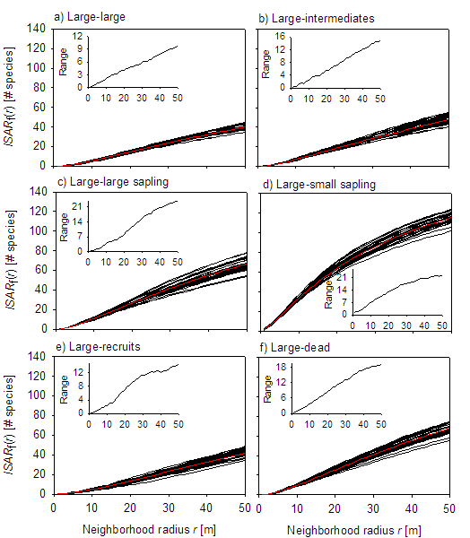
Fig. A1. The observed ISAR functions (black lines) for the different size class combinations together with the mean of all observed ISAR curves (red line). The small insets show the range of the observed ISAR functions at the different neighborhoods (i.e., the difference between the maximal and the minimal observed ISAR values). Results are for the second census.

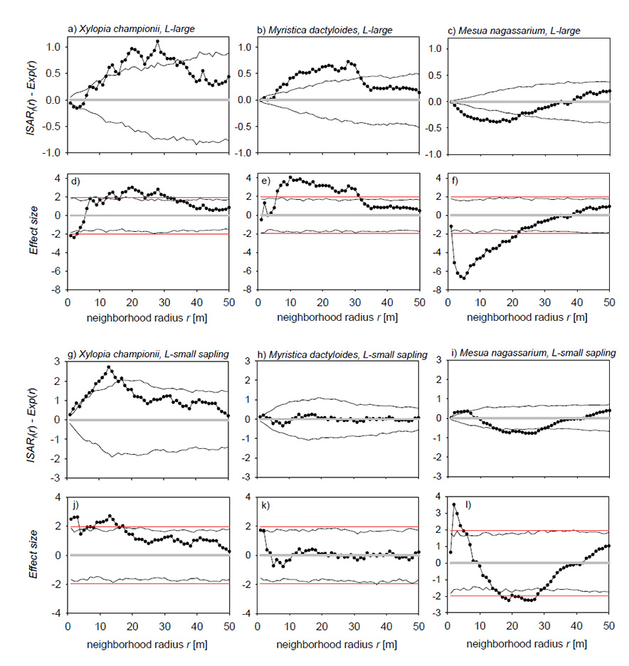
Fig. A2. Examples for the ISAR function and their effect sizes for three species. (a) – (c) Analysis of species richness of large trees around large trees. Difference between observed ISARf(r) and the expectation Exp(r) under the independence null model as function of neighborhood radius r (closed circles) and corresponding simulation envelopes (black lines). (d) – (f) Same as (a) – (c), but effect size transformation [ISARf(r) - Exp(r)]/SD(r) (closed circles), corresponding simulation envelope (black line) and theoretical expectation of simulation envelope (-1.96 and 1.96; red lines) for a significance level of α = 0.05. SD(r) is the standard deviation of the 199 simulations of the independence null model. Effect sizes < -1.96 indicate repeller effects and effect sizes > 1.96 indicate accumulator effects. Results are for the second census. (g) – (l) same as (a) – (f), but for the analysis of species richness of small saplings around large trees.

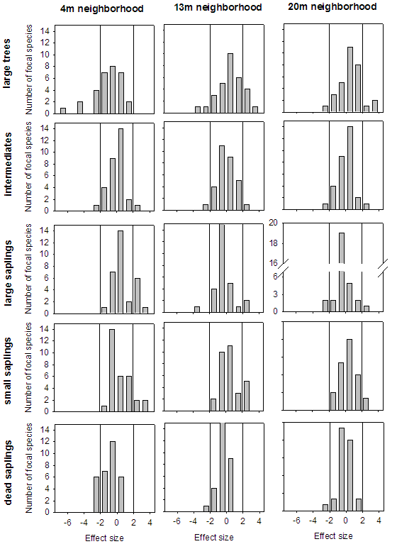
Fig. A3. Distribution of effect sizes for different spatial scales (columns) and different size classes (rows). The vertical lines indicate the range (-1.96, 1.96) where the effect size is not significant at a 5% confidence level. Effect sizes < -1.96 indicate repeller effects and effect sizes > 1.96 indicate accumulator effects. Results are for the second census.

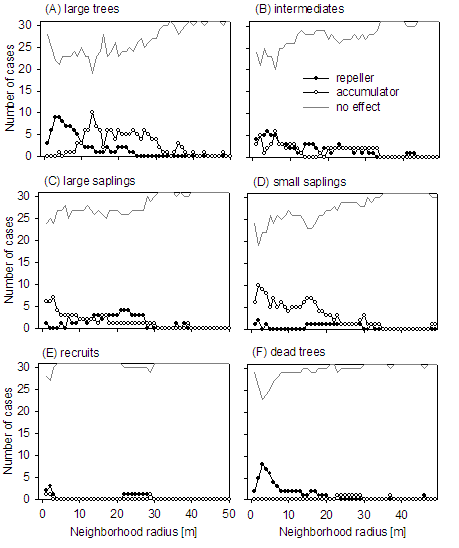
Fig. A4. Same as Fig.1, but for the second census period. 31 focal species were analyzed.

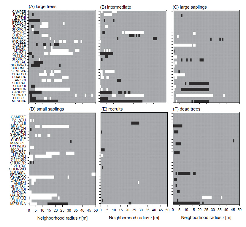
Fig. A5. Same as Fig. 3, but for the second census period where 31 focal species were analyzed.

Table A1. Number of individuals in the different size classes.

Table A3. Same as Table A2, but for analysis of the community of small trees around large focal trees.

Table A4. Paired two sample sign test for testing the uniqueness of diversity sequence for two species (as an example).

Row values for Species X and Species Y: 0 for no effect species, 1 for accumulator species, and -1 for repeller species at distance r meter (1–25 m). We used paired two sample sign test to test whether these two sequences are significantly different or not. |Difference| is measured by the absolute difference of (|SpeciesX-SpeciesY|). Our null hypotheses was median = |Difference| = 0.

Table A5. Paired two sampled sign test for testing the degree of uniqueness of the diversity sequence for each pair of large trees of focal species at 1–25 m spatial scale (α = 0.05 significant levels) for the second census. sp: species number.

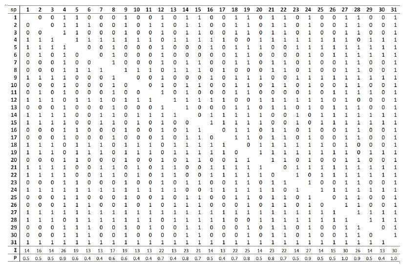
Table values: 1 for neighborhood diversity of two focal trees is significantly different, 0 for not significantly different, Σ is the number of large trees of focal species that are significantly different to the given focal species. P is the proportion of large trees of focal species that are different to the given focal species. P is a measure of the degree of uniqueness of neighborhood diversity of the focal species (vary from 0–1). For example, see species in column 27 and 31 (i.e. M. dactyloides  and M. nagassarium ). These two species are significantly different from all the other species. Full names for species index sp follows species names listed in Table 2.

Table A6. Paired two sample sign test (see Table A4) for testing the difference of neighborhood diversity of trees in the small saplings vs. large trees around large trees of focal species at (1–25 m) for the second census. Species for which the species richness of the large trees was larger than expected (accumulator species) are indicated by yellow color, those for which species richness was lower than expected (repeller species) are indicated by blue color and those with no departure from the independence null model (no effect species) are indicated by gray color.

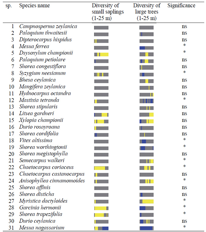
*: significant, ns: not significant (α = 0.05 significant level)

[Back to E096-164]