![]()
Ecological Archives E096-161-A1
Jerod A. Merkle, Seth G. Cherry, and Daniel Fortin. 2015. Bison distribution under conflicting foraging strategies: site fidelity vs. energy maximization. Ecology 96:15031511. http://dx.doi.org/10.1890/14-0805.1
Appendix A. Details of the abundance model used to estimate annual population size.
A.1 GPS collar data
We monitored a total of 57 adult female (> 3 years old) bison during the study using GPS radio collars (GPS 1000 and CanadaGPS collar 4400M, Lotek Engineering, Newmarket, Ontario; Telonics Argos, Telonics, Mesa, Arizona, USA). Captures were conducted in late winter using a helicopter. Collars deployed between 1996 and 1999 were programmed to take 8 locations per day. Collars deployed between 2005 and 2013 took 8 locations per day for 5 days, and 24 locations per day 2 days per week. We monitored individuals until death, collar malfunction, or battery exhaustion. Individuals collared in the 1990s were monitored for 285 ± 225 days ( ± SD) with a fix success rate ca. 60%. We monitored individuals in the 2000s for 777 ± 511 days with a fix success rate of > 96%.
A.2 Annual bison survey
In 1995, Parks Canada officials developed a bison monitoring protocol. Thirty-one transects paralleling the southern PANP boundary were superimposed over the bison range. Transect spacing was stratified to more intensively search within the estimated core range, which was determined by opportunistic ground observations and preliminary aerial surveys. The eleven northern and seven southern transects were spaced 1.5 km apart, and the middle thirteen transects in the core were spaced 1.0 km apart (Fig. B1). Transects were on average 20 km long. Annual surveys were conducted in late winter (mean date was 3 March) using a helicopter at an altitude of 250 m with 2 observers in the back (one on each side) and a data recorder in the passenger seat. When bison were observed, personnel either noted the Global Position System (GPS) location on the transect line or manually located the group on a topographic map with the transect lines. For the latter, GPS locations of bison groups were obtained by superimposing the maps in a geographical information system program. Personnel also noted the time, whether or not bison were on the north or south side of the survey line, and whether they were within 250 m of the transect using a gauge traced on the windows of the helicopter.
A.3 RSF for abundance model
We integrated changes in annual behavior related to detection probability during aerial surveys into our abundance model by parameterizing a Resource Selection Function (RSF) at the 2nd order scale (Manly et al. 2002). In developing the RSF, we used GPS location data collected five weeks before, and five weeks after aerial survey dates.
For each observed GPS location, we generated a random matched location for comparison within the entire bison range. We calculated the entire bison range using kernel density estimators for all the collar and survey location data. Using a 100 m resolution grid and the reference technique to estimate the smoothing factor (h = 1,200 m), we calculated a bivariate normal kernel (Worton 1989) of all GPS radio collar locations collected at three hour increments throughout the study (n = 181,854). Using the same grid and smoothing factor estimation method (h = 2,757 m), we also calculated a bivariate normal kernel of all locations of individual or groups of bison seen during aerial surveys (n = 477). We calculated a contour for each kernel that represented a single polygon without gaps (i.e., 99% and 95% for the collar and survey data, respectively). The overall range was then calculated as the total area (959 km²) encompassing both contours.
We identified land cover types for observed and random locations using classified Landsat Enhanced Thematic Mapper satellite images (28.5 m resolution) collected in August 2001 (Fortin et al. 2009). The 18 landscape cover types originally identified were combined to form 3 more general cover types relevant to aerial detectability of bison in winter: open (i.e., meadow, agriculture, shrub, roads, water, bare ground), coniferous (i.e., conifer, mixed conifer and deciduous forest), and deciduous (i.e., deciduous forest, riparian). During parameterization, deciduous forest was withheld as the reference category. We assigned distance (in km) from the nearest survey line to each observed and random location to allow for annual variation in the spatial distribution of bison on probability of detection during surveys. To obtain parameter estimates for each year, we specified a random intercept and random slopes for each variable based on each year represented in the analysis. Parameterization of the RSF for the abundance model was conducted using a generalized linear mixed effect model with a binomial distribution in the lme4 package in R version 3.0.2 (R Core Team 2014).
A.4 Abundance model
We estimated annual population size using a generalized N-mixture model (Dail and Madsen 2011), allowing for an unbiased estimator when animals immigrate and emigrate among sites between surveys (such as our case). Using migration decomposition (Royle 2004), the generalized N-mixture approach models abundance at site i and time t, Nit, as the sum of two random variables Sit and Git, multiplied by detection probability p. Sit denotes animals in site i at time t who survived and stayed in that site since t – 1 (i.e., apparent survival), and Git denotes gains (or arrival rate) at site i since t – 1 (i.e., apparent recruitment). Because the model is based on unmarked individuals, we use the word “apparent” because it is not possible to distinguish between losses due to mortality or emigration, or between gains due to births or immigration from another site. For Ni1, the model is based on λ, or an initial abundance at each site at t = 1. The hierarchical model and distributions in our case took the following forms: Ni1 ~ Poisson(λ), Sit ~ Binomial(Nit-1, ω), Git ~ Poisson{ f(γ; Nit-1)}, Yit ~ Binomial{Nit, f(p; Xt)}, where ω is the probability of surviving and staying given the previous year’s abundance, f(γ; Nit-1) is the apparent recruitment rate based on a function of the previous year’s abundance, Yit is the observed aerial survey count data for each site i and time step t, and f(p; Xt) is the detection probability based on a function of an array of covariates X at each time step t.
We assumed there was a baseline apparent recruitment rate within a site (γ0), or a rescue effect, independent of Nit-1. We also assumed that apparent recruitment would vary based on the parameter γ1 dependent on Nit-1, given a log link function: f(γ; Nit-1) = exp(γ0 + γ1 × Nit-1). We included how annual RSF coefficients affected detection by incorporating the following logistic function for detection probability p for each site i and year t:
where p0 is the baseline detection probability and p1…p3 correspond to the effect of annual variation in habitat selection based on mean selection coefficients, β1t…β3t, obtained in the RSF analysis above. We based the generalized N-mixture model on 3 sites corresponding logically to the northern, central, and southern transects.
We parameterized the generalized N-mixture model using Markov chain Monte Carlo (MCMC) techniques within a Bayesian framework. We specified uninformative priors for all parameters except for baseline capture probability (p0). We identified a range of detection probabilities for p0 using a four-step process where we estimated the proportion of collared individuals that were counted during aerial surveys (n = 50). First, during surveys where bison observations were noted on the transect line, we added or subtracted 250 m from the northing coordinate of the observation based on whether bison were seen outside the 250 m mark and whether they were seen north or south of the survey line. Second, we developed buffers around the locations of bison observations during surveys of 600 to 1500 m (in increments of 100 m), allowing for a number of observation error sources. These include error from, (1) locations recorded just before or after the helicopter passed the observed bison (i.e., not perpendicular to the survey line), (2) bison observed > 250 m from the transect line and the distance was not specified, and (3) geo-referencing from topographical maps to GPS coordinates. Third, we approximated the locations of collared animals at 10 minute intervals during each survey using a Brownian Bridge movement simulation between fixes (Horne et al. 2007). Finally, we calculated the percent of collared animals observed during surveys by examining whether bison observations during surveys overlapped with actual and simulated locations of collared bison in space (i.e., whether or not locations of collared animals were within the survey observation buffer) and time (whether or not locations of collared animals were within 15 minutes of recorded bison observations during surveys). We repeated the process 1,000 times to allow for variation in the simulation of movement paths. We used the resulting minimum and maximum estimated detection percentages (60% to 82%) as bounds for a uniform prior distribution on p0 in the abundance model.
For parameter estimation, we ran three parallel MCMCs with a burn-in of 10,000 iterations. We generated posterior samples using 25,000 iterations of the model and a thinning rate of 25. We chose the number of iterations by calculating the Gelman and Rubin convergence diagnostic (Brooks and Gelman 1998). We chose the thinning rate by examining autocorrelation plots of the MCMC chains, and increasing the thinning rate until no correlation among parameter values was observed. Parameterization of the generalized N-mixture model was conducted in R and JAGS (Plummer 2003) using the R package rjags.
A.5 Validation of abundance model
We used an additional independent means of estimating bison population size to validate the accuracy of our N-mixture abundance model. During summer, bison in our study area spend most of their time in a small core area made up of a network of meadows (approx. 100 km²), most of which are accessible by trail. During summers (i.e., May to first week of August) 2011–2013, we developed circuits (i.e., trail networks containing meadows frequently used by bison) where we searched for bison. Each circuit was completed 2–6 times per week (i.e., depending on weather and logistics), keeping effort consistent within each summer. While surveying the circuits we searched for bison groups in meadows, and when found, we opportunistically took photographs of the faces of as many adult bison (3 years old and older) as possible and noted group composition (i.e., no. adult males, adult females, juveniles [yearlings and two-year olds], and calves). Following the methods of Merkle and Fortin (2014), we identified individual animals from photographs using a likelihood-based image matching approach, where we extracted measurements of phenotypic characteristics of bison horns and used an algorithm that helps identify matches. From the database of matched individuals, we developed capture histories based on 10, 14, and 12 sampling events, corresponding to each week during summers 2011, 2012, and 2013, respectively. Using program MARK (White and Burnham 1999), we estimated adult population size for males and females following the methods of Merkle and Fortin (2014).
Finally, we estimated total population size for each year by combining estimates of the number of adult males and females, juveniles and calves. First we estimated the calf- and juvenile-cow ratio using a binomial distribution, where we estimated the intercept of a model describing the daily cow-to-calf or -juvenile ratio observed, weighted by the number of cows observed throughout a day (i.e., if multiple groups of bison were seen on one day, those numbers were combined). We only used counts from June to August because prior to June, females with calves were sometimes observed alone. We calculated total population size of bison along with 95% confidence intervals using a simple bootstrapping procedure (Efron and Tibshirani 1986), where we resampled each estimate (males, females, and juvenile and calf-to-cow ratios) 1,000 times based on a normal distribution with the mean as the estimate and the SD as the SE. In validating our abundance model, we reported the degree to which the confidence intervals of estimates from the Generalized N-mixture and photographic mark-recapture models overlapped.
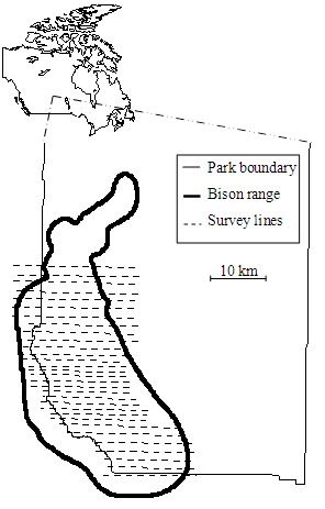
Fig. A1. The study area, depicting the plains bison range located in and around the southwestern portion of Prince Albert National Park, Canada, and the transect lines used for surveying plains bison during winters 1996–2013.
Literature Cited
Brooks, S. P., and A. Gelman. 1998. General methods for monitoring convergence of iterative simulations. Journal of Computational and Graphical Statistics 7:434–455.
Dail, D., and L. Madsen. 2011. Models for estimating abundance from repeated counts of an open metapopulation. Biometrics 67:577–587.
Efron, B., and R. Tibshirani. 1986. Bootstrap Methods for Standard Errors, Confidence Intervals, and Other Measures of Statistical Accuracy. Statistical Science 1:54–75.
Fortin, D., M. E. Fortin, H. L. Beyer, T. Duchesne, S. Courant, and K. Dancose. 2009. Group-size-mediated habitat selection and group fusion-fission dynamics of bison under predation risk. Ecology 90:2480–2490.
Horne, J. S., E. O. Garton, S. M. Krone, and J. S. Lewis. 2007. Analyzing animal movements using Brownian bridges. Ecology 88:2354–2363.
Manly, B. F. J., L. L. McDonald, D. L. Thomas, T. L. McDonald, and W. P. Erickson. 2002. Resource selection by animals. Second edition. Kluwer Academic Publishers, Dordrecht, the Netherlands.
Merkle, J. A., and D. Fortin. 2014. Likelihood-based photograph identification: application with photographs of free-ranging bison. Wildlife Society Bulletin 38:196–204.
Plummer, M. 2003. JAGS: A program for analysis of Bayesian graphical models using Gibbs sampling. Pages 20–22 in Proceedings of the 3rd International Workshop on Distributed Statistical Computing (DSC 2003), Vienna, Austria.
R Core Team. 2014. R: A language and environment for statistical computing. R Foundation for Statistical Computing, Vienna, Austria.
Royle, J. 2004. Generalized estimators of avian abundance from count survey data. Animal Biodiversity and Conservation 27:375–386.
White, G. C., and K. P. Burnham. 1999. Program MARK: survival estimation from populations of marked animals. Bird Study 46:S120–S139.
Worton, B. J. 1989. Kernel methods for estimating the utilization distribution in home-range studies. Ecology 70:164–168.