Ecological Archives E096-156-D1

Jonathan P. Dandois, Dana Nadwodny, Erik Anderson, Andrew Bofto, Matthew Baker, and Erle C. Ellis. 2015. Forest census and map data for two temperate deciduous forest edge woodlot patches in Baltimore, Maryland, USA. Ecology 96:1734. http://dx.doi.org/10.1890/14-2246.1

Introduction

Forests cover roughly 30% of global land area and hold 70–90% of terrestrial aboveground and belowground biomass, a key sink of global carbon (FAO and JRC 2012). Globally forests are experiencing increased disturbance pressure due to changes in climate, water and nutrient cycles as well as changes in land use (Foley et al. 2005). Understanding how forests will be effected by such pressures requires long-term monitoring over the same forested areas to track dynamics through time. The long-term forest plots established by the Center for Tropical Forest Studies Forest Global Earth Observatory (CTFS-ForestGeo) represent the largest global network of research sites established and maintained for the purpose of tracking forest change (Anderson-Teixeira et al. 2014). Regular re-census of these plots provides valuable information on forest demography and the response of the forest to disturbance pressures. Even so, many of the 59 forest plots within this network are located within mature or secondary intact forests, often within national parks or other protected biological reserves (Anderson-Teixeira et al. 2014).

Remote sensing-based studies suggest that, instead of consisting of large uninterrupted swaths of land, significant portions of forest area at regional and global scales exist within fragmented landscapes, characterized by relatively higher proportions of edge than interior forest area (Riitters et al. 2000, Riitters et al. 2002). Those located within urban and suburban areas (herein: 'urban forests') are found embedded within a patchwork mosaic of built surfaces, open fields, agricultural areas and other kinds of land use (Ellis and Ramankutty 2008, Potere et al. 2009). However, the altered position of urban forests within the landscape does not undermine their value relative to larger, intact forest areas. Urban forests provide many ecosystem services to the local environment and the people living nearby, including mitigating energy costs, heating, and water runoff, as well as providing habitat, fuel and fiber (Costanza et al. 1998, Dwyer et al. 1992, McPherson et al. 1997, Bolund and Hunhammar 1999). Urban forests experience a wide range of disturbances that might not be experienced at long-term forest monitoring sites embedded within intact forests, parks, and reserves. Wildlife in urban forests may experience increased pressure from pets (cats, dogs) from nearby housing areas (Lenth et al. 2006, Loyd et al. 2013). Forest patches within urban areas may also be criss-crossed by pedestrian trials and even experience regular mowing of understory vegetation (Hobbs 1998). Improving understanding of how forests within urban ecosystems will change under local and global-scale pressures requires long-term monitoring efforts (Pickett et al. 2001). Permanent urban forest plots that are re-censused based on established protocols will provide an invaluable resource for understanding the response of these important forest areas to local and global-scale disturbance pressures.

This data paper provides a description of the first census of two Temperate Deciduous forest patches within a suburban landscape mosaic on the campus of the University of Maryland Baltimore County (UMBC) in Baltimore MD USA carried out between 2012–2014. Data on the location, diameter at breast height (DBH), condition (e.g., alive/dead, multiple stem, etc.,) of all stems ≥ 1 cm DBH for two 6.25 ha (250 m × 250 m) permanent forest census plots are organized based on the Smithsonian Tropical Research Institute CTFS-ForestGeo data protocol.

This data set was initially developed to provide reference measurements of forest understory and canopy physical structure for comparison against novel computer vision remote sensing observations obtained from the air by unmanned aerial systems (UAS; Dandois and Ellis 2013) and by an individual walking on the ground through the forest and taking pictures with a cell phone or mobile tablet computer (NSF Grant DBI 1147089 awarded 1 March 2012 to Erle Ellis and Marc Olano). High spatial resolution remote sensing of vegetation structure in three-dimensions (3D) has become an important tool for a broad range of scientific and environmental management applications, including national and local carbon accounting (Frolking et al. 2009, Goetz and Dubayah 2011, Houghton et al. 2009) and serves as a core data product of the National Ecological Observation Network (NEON; Schimel et al. 2011). Adding to this, measurements of canopy 3D structural and spectral traits by automated computer vision and regular digital cameras offers the potential to capture forest structural and spectral seasonal dynamics at the scale of individual trees (Dandois and Ellis 2010, 2013), a technique that could even by employed by individuals strolling through a forest taking pictures with a cell phone (Turner 2014). While the broad goal of remote sensing is to provide a replacement or at least comparable substitute for costly and labor intensive field surveys, inferences about ecosystem traits from remote sensing data, whether from established or new techniques, still require some evaluation against 'gold-standard' or 'ground-truth' field-based observations (Defries et al. 2007; Dubayah et al. 2010; Frolking et al. 2009). Spatially explicit ground-truth information is required for improving remote sensing-based estimates of local and regional forest biomass density, forest composition and type, and for parameterizing ecosystem models that use remote sensing data.

This data set and subsequent re-census following ForestGeo protocols will provide valuable information about the structure and demography of urban forest patches. Regular re-census of these plots will make it possible to track turnover of understory and overstory species density and dominance and also changes in the composition and structure at the forest edge where disturbances are highest. For example, the aggressive, bird-dispersed vine English Ivy (Hedera helix) is found in abundance within these plots and in the surrounding landscape. Along with overcoming and killing-off host trees, the presence of H. helix can dramatically alter forest physical structure, creating a potential barrier to dispersal of native species (Cadenasso and Picket 2001, Vidra et al. 2006). Regular re-census can help to shed light on the patterns and processes of invasion and dispersal within urban forest patches. This data set provides an excellent complement to the other long-term forest monitoring sites within the ForestGeo network as it captures a forest type and disturbance regime that is not captured at other sites which are located within intact forests, parks, and reserves. Because this data set provides spatially explicit information on tree species and tree size (stem locations are reported in the Universal Transverse Mercator, UTM, projected coordinate system) it can be used as ground-truth reference for airborne and satellite remote sensing observation.

The original data publication reflects the first census conducted between 2012–2014. The most up-to-date version can be found at http://www.forestgeo.si.edu/. Additional information about the Ecosynth project for which this data was collected can be found at http://ecosynth.org.

Metadata

Class I. Data set descriptors

A. Data set identity: UMBC Campus Permanent Forest Inventory Plots, Baltimore, MD, USA.

B. Data set identification code: ----

C. Data set description

Originaors: Jonathan P. Dandois UMBC GES, 1000 Hilltop Circle, Sondheim 211, Baltimore MD 21250, USA (Post-doctoral research fellow, Smithsonian Tropical Research Institute, Panama; [email protected]) Dana Nadwodny Erle C. Ellis, UMBC GES, 1000 Hilltop Circle, Sondheim 211, Baltimore MD 21250, USA (Associate Professor; [email protected]).

Abstract: This data set reports on a census of all trees within two 6.25-ha plots (250 m × 250 m) of temperate deciduous woodlot patch on the campus of the University of Maryland Baltimore County (UMBC), Baltimore, Maryland, USA. Woodlot patches are primarily of the tulip poplar association. From 2011–2012, a 25 m × 25 m quadrat grid was established for each plot by total station surveying equipment. From 2012–2014, the location and DBH (diameter at breast height, 1.37 m) of all woody stems ≥ 1 cm DBH that reached ≥ 1.37 m tall were censused, whether living or dead. All such stems were also marked with numbered metal tags. All living stems were identified at least to genus and to species when possible. All censused stems and associated data (tag number, DBH, location, species, status) were entered into a geographic information system (GIS) map layer based on stem location within a Universal Transverse Mercator (UTM) projected coordinate system where each stem was represented as a unique point feature. The primary objective of these data is to provide a reference for stem location and diameter for the calibration and evaluation of ground-based 3D remote sensing technologies based on computer vision and personal digital camera or cell phone image collections. With regular re-census, the data could also be used for tracking growth, mortality, and recruitment of patchy forest woodlots within a suburban landscape mosaic.

D. Key words: deciduous; diameter; Ecosynth; forest inventory; map; patch; species; survey; taxonomy; temperate; urban forest.

Class II. Research origin descriptors

A. Overall project description

Identity: Ecosynth: An Advanced Open-Source 3D Toolkit for Forest Ecology

Originators: Erle C. Ellis, UMBC GES, ([email protected]). Marc Olano, UMBC CSEE, ([email protected]). 1000 Hilltop Circle, Sondheim 211, Baltimore MD 21250, USA

Period of Study: Ongoing since 2010

Objectives: Develop, demonstrate and promote "Ecosynth", an open-source 3D toolkit for scanning woodland ecosystems based on computer-vision technologies coupled with a community online system for browsing, sharing, visualizing, tagging and analyzing 3D scans of terrestrial ecosystems.

Abstract: Woodlands are currently targeted for carbon and biodiversity conservation by REDD+ and other international agreements and are therefore key areas for expanded scientific research and monitoring. Enabling regular inexpensive use of 3D imaging tools by field ecologists and citizen scientists will expand forest observation capabilities to a much wider pool of observers, thereby assisting in global forest conservation efforts and even urban forestry. The project is built upon an interdisciplinary team from multiple disciplines: ecology, geography, math, computer science, electrical and mechanical engineering, and information systems. Ultimately the project aims to spark the development of an open source 3D ecology community dedicated to developing, sharing and investigating the ecology of woodlands based on the results of 3D scanning using computer vision. The forest inventory data set presented here provides the ground-truth reference for such 3D observations and in doing so characterizes the structure of two Temperate Deciduous forest patches within a suburban / institutional landscape.

Sources of funding: Forest structure research was supported by USDA Forest Service Joint Venture Agreement 06-JV-11242300-135, awarded to Erle Ellis in 2010. This material is based upon work supported by the US National Science Foundation under Grant DBI 1147089 awarded March 1, 2012 to Erle Ellis and Marc Olano. Jonathan Dandois was supported by NSF IGERT grant 0549469, PI Claire Welty and hosted by CUERE (Center for Urban Environmental Research and Education).

B. Specific subproject description

Site description: (Dandois and Ellis 2010, 2013).

Site type: Liriodendron tulipifera tulip poplar association forest (Brush et al. 1980).

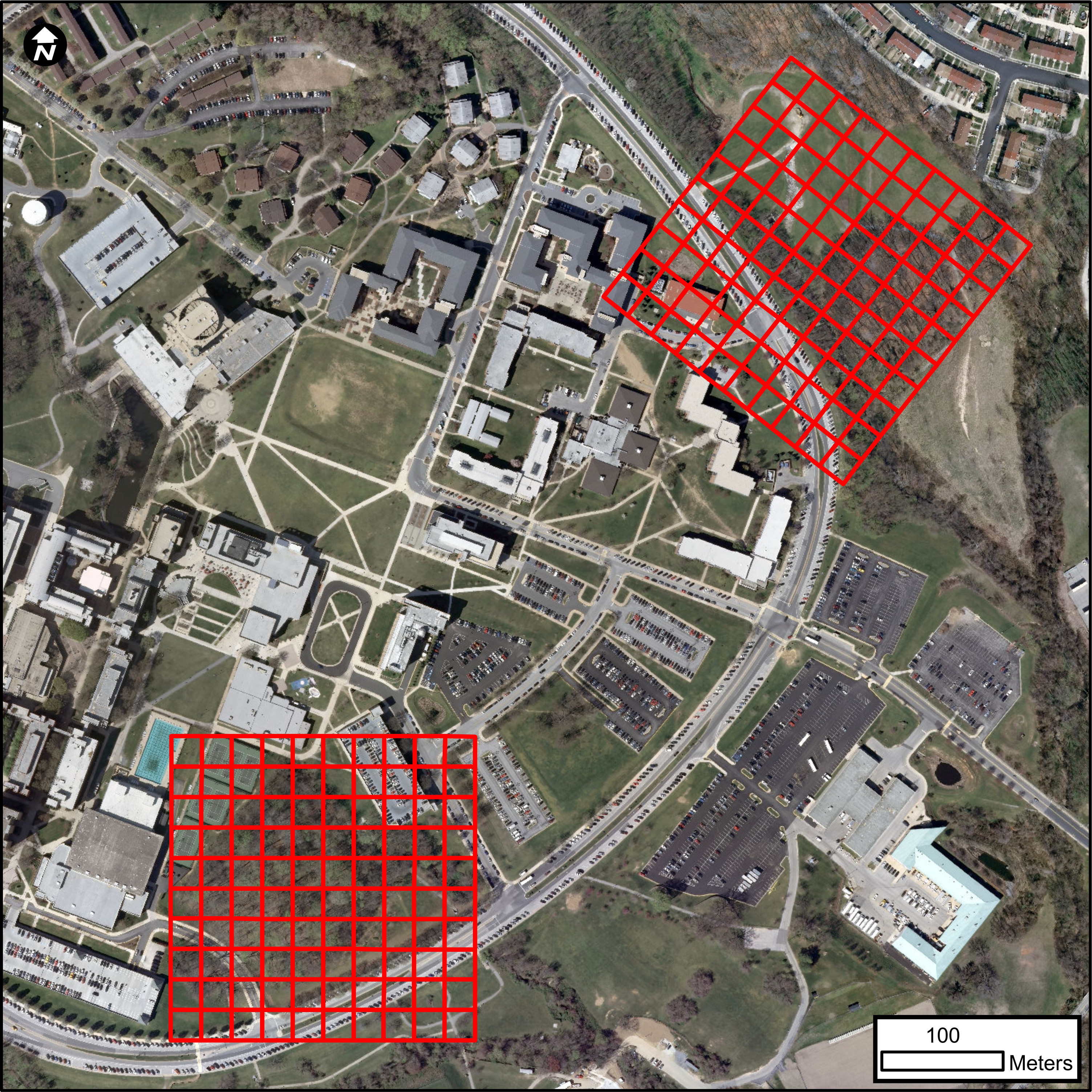
Geography: Census plots are 250 m × 250 m (6.25 ha) in size and are located on the campus of the University of Maryland Baltimore County situated ca. the boundary of the Piedmont Plateau and Coastal Plain (Brush et al. 1980). UMBC, Baltimore, Maryland, USA, ca. 39.25500°, -76.70889°, altitude between 40 and 60 m above mean sea level (Fig. 1).

Fig. 1: Location map of 250 m × 250 m UMBC census plot quadrat grids: Knoll (KN; lower) and Herbert Run (HR; upper) on the UMBC campus. Image source: 2008 leaf-off aerial orthophotograph (Baltimore County Office of Information Technology; Sanborn Map Company, Inc., Colorado Springs, CO; 0.6 m horizontal accuracy, 0.3 m pixel resolution; collected 2008/03/01 – 2008/04/01).

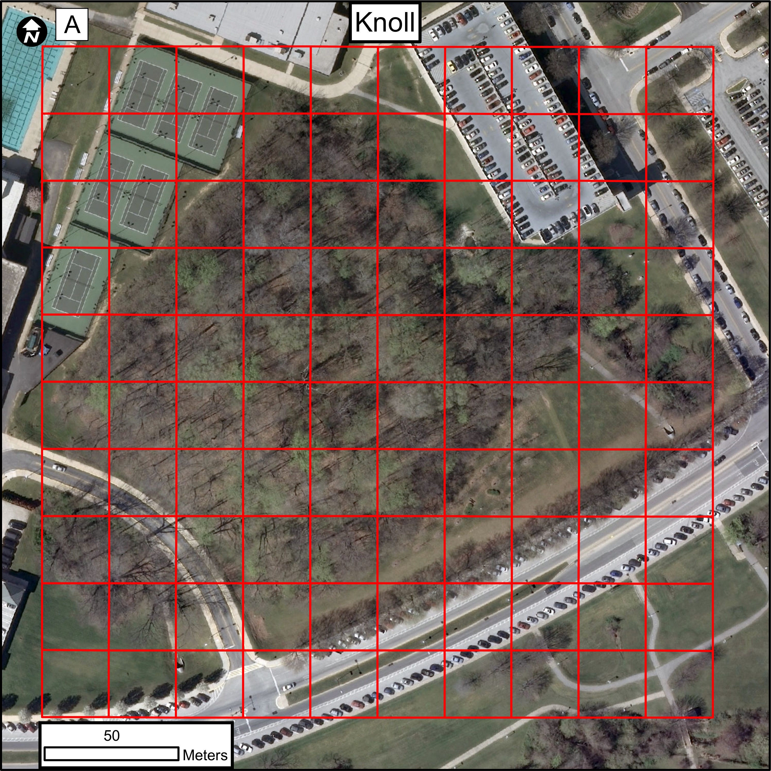
Habitat:We conducted forest inventories at two sites located on UMBC Campus: Herbert Run and the Knoll. The Knoll (Fig. 2a) is a forested hill located on UMBC campus (ca 39.252592° -76.710408°) and is a mixed-age forest composed primarily of American beech (Fagus grandifolia), oak (Quercus spp.), and hickory (Carya spp.). Additionally there are many mature white ash (Fraxinus americana) and tulip poplar (Liriodendron tulipifera). 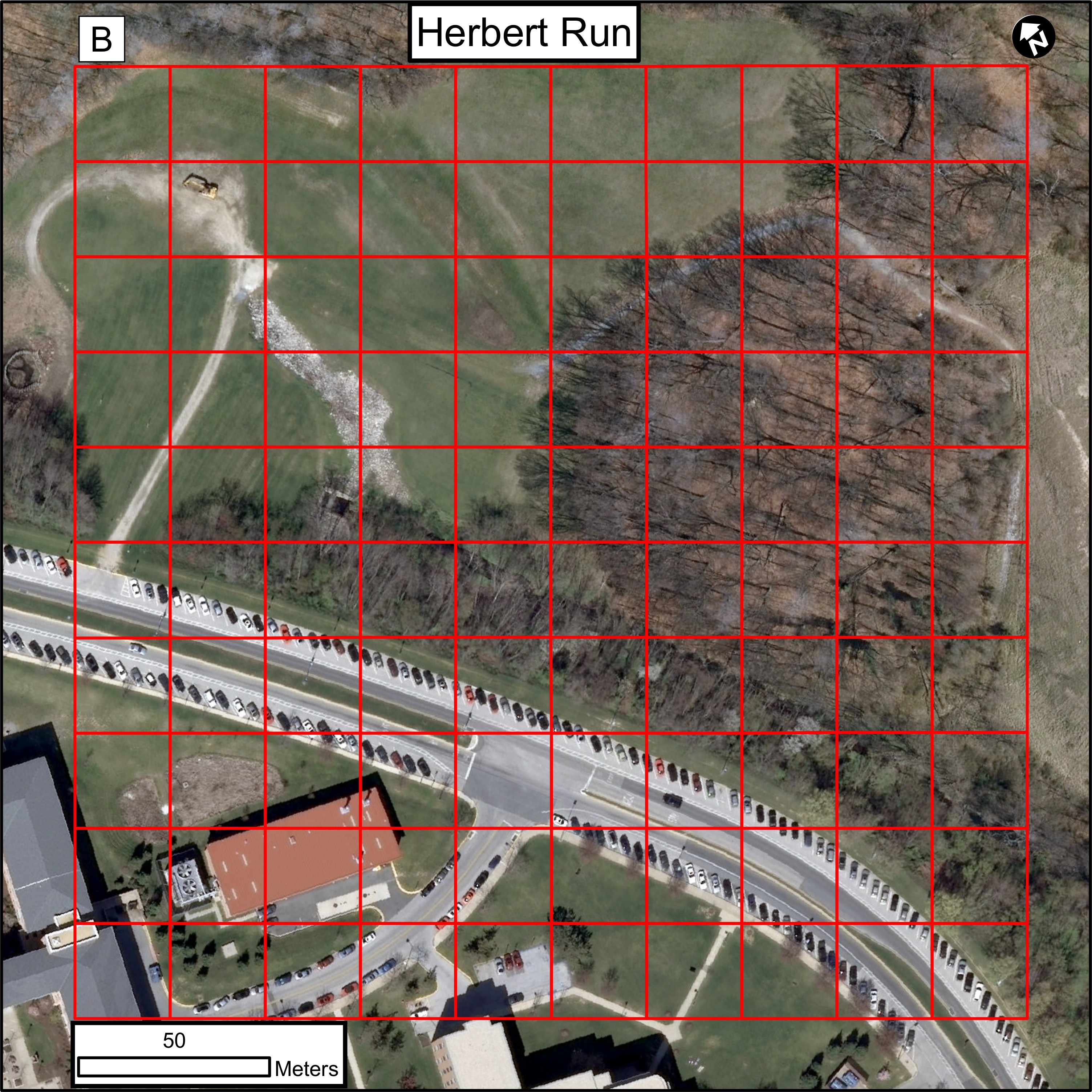Herbert Run (Fig. 2b, ca 39.257187° -76.705748°) is characterized by a remnant woodlot patch of similar age and composition as the Knoll, which is adjacent to a steeply sloping (grade up to 50% in some places) secondary forested riparian zone along a stream and adjacent to a road. This secondary forest is composed mainly of an even-aged stand of black locust (Robinia pseudoacacia) and black cherry (Prunus serotina) along the steep stream banks. In close proximity to the stream honey locust (Gleditsia triacanthos) and green ash (Fraxinus pennsylvanica) become more prevalent.

Fig. 2: Zoomed in view of 250 m × 250 m plot quadrat grids over the Knoll (2A, left) and Herbert Run (2B, right) plots at UMBC. Image source: see Fig. 1.

Geology, landform: UMBC is located roughly along the boundary between the Piedmont Plateau and Coastal Plain geologic provinces (Brush et al. 1980). Soils at both plots can be characterized as a mix of Urban in-fill and sandy to silty loams of Russett and Keyport composition (Natural Resources Conservation Service, NRCS, http://websoilsurvey.nrcs.usda.gov, accessed: 2014/06/13).

Watersheds/hydrology: Both plots are located within the watershed of Herbert Run, a tributary of the Patapsco River, which feeds into the Chesapeake Bay.

Site history: Both plots are located within institutional land use of UMBC. The main patch of the Knoll site is a remnant woodlot from a period of agricultural land use that preceded the establishment of UMBC ca 1966. Roughly 60% of the forest area at Herbert Run is of the same history as the main patch at the Knoll. Aerial photo-interpretation places the age of both main woodlot patches at > 75 years old: patches were visible with similar extents in an aerial photo dated 1938. Forest along the Herbert Run stream and adjacent to the road Hilltop Circle has regrown on infill soil after road construction. Table 1 describes the proportion of land cover at each 6.25 ha plot as of the date of the initial census (August 2014). Land cover at both sites was manually interpreted and digitized in ArcGIS 10.0 (ESRI, Redlands, CA) from a 2008 leaf-off aerial orthophotograph (Baltimore County Office of Information Technology; Sanborn Map Company, Inc., Colorado Springs, CO; 0.6 m horizontal accuracy, 0.3 m pixel resolution; collected 2008/03/01 – 2008/04/01) into seven categories: forest (woody vegetation >2 m height), turfgrass, brush (woody vegetation < 2 m height), buildings, pavement, water, and other (i.e., rock rip-rap, unpaved trail). Land cover feature height (e.g., greater or less than 2 m) and aboveground feature outline (e.g., for buildings and forest canopy) was determined from a 1 m resolution three-dimensional canopy height model for which each pixel value refers to the height above ground of the tallest surface within that pixel (collected 2010/10/06 – 2010/10/08; Dandois and Ellis 2013). Accuracy of land cover interpretation was by field visit and was determined to be correct as of the date of the initial census. See Dandois and Ellis (2013) for details on classification methods.

Table 1: Percentage of land covers within each 6.25 ha plot at UMBC as of August 2014. Land covers determined by aerial photo-interpretation.
	Forest	Turf grass	Brush /Tall Grass	Buildings	Pavement	Water	Other / Bare
Knoll	55 %	20 %	--	5 %	20 %	0.1 %	--
Herbert Run	44 %	37 %	1 %	2 %	14 %	--	2 %

Social and ecological context of sites: While both sites have remained as more or less in-tact patches of forest over the last 75+ years (based on aerial photo interpretation) they regularly experience strong disturbance pressures from the local community. Both sites are surrounded by non-forest land use and land cover, contain small foot paths, and 'hang-out' areas with trampled ground, trash and other forms of disturbance (tree carving, rope swings). During one field visit, a metal cable zip-line was observed at the Hebert Run site that crosses the shallow ravine over the Herbert Run stream. Throughout field surveys, we frequently saw evidence of small campfires at both sites. Animals seen at the sites include: white-tail deer (Odocoileus virginianus), gray squirrel (Sciurus carolinensis), red fox (Vulpes vulpes), snapping turtle (Chelydra serpentina), black rat snakes (Pantherophis obsoletus) as well as many bird species common to the area. There is also a signifcant invasion of the aggressive, bird-dispersed vine English Ivy (Hedera helix) at both sites. While vines were not included in the initial census, their presence could be noted in future re-census of the sites.

The Knoll site is completely surrounded by campus development and is a forest island surrounded by roads, buildings, parking garages, and tennis courts. A small park/garden next to the Knoll patch contains park benches and several planted red oaks (Quercus rubra). At the northern edge of the plot a storm drain empties into a stream which joins the Herbert Run stream that runs through the campus. Re-enforcing of the storm drain outflow resulted in several trees being removed and new saplings planted along the disturbed area (< 1 cm DBH at the time of census). Several small pedestrian trails criss-cross the main patch and are used by students that cut through the forest to walk between parking areas and campus buildings or to enter the patch itself. The site is located directly adjacent to the campus athletic facilities and tennis courts. Tennis balls and trash are frequently found within the forest edge near the courts and the lights often remain lit over the courts until 22:00. While the patch is considered an important "green" asset of the campus area, it is not entirely protected. Beginning in August 2014 and at the end of the first census period, a small isolated patch of forest (roughly 0.25 ha) with a small stream fed by a storm drain was completely clear cut and the land completely raised and reformed in preparation for new road construction.

The Herbert Run site abuts a campus road but is also adjacent to a medium density townhouse complex. To the north of the patch is a large open field of man-made landform, formed for the creation of an earthen flood control dam over the Herbert Run stream which is visible in Figure 1b where an unpaved road enters the field from the main campus road. Grass in this field is cut weekly, however we are not aware that it is ever fertilized. The field is often used by athletic groups and both the field and the forests in this area are frequented by dog walkers, particularly from the nearby apartment complex. At least one other storm drain from the campus empties directly into the Herbert Run within the plot area. At the north-east edge of the Herbert Run plot runs a chain-link fence maintained by University personnel to prevent residents from the neighborhood from entering the property. To the south-east of the patch is a large man-made hill formed on fill dirt from campus construction and which is covered with a mix of unmanaged tall (> 0.5 m in summer) grasses. The hill is accessed by an old asphalt road that cuts through the forest and which is visible in the aerial photos in Fig. 1b. At the time of the first census, this road was frequently in use by construction trucks to dump or remove dirt from the hill in association with new campus construction. To the south-west of the Herbert Run patch and within the plot area is a small water retention pond and over 50 planted trees around campus buildings of species not found in any other parts of the forests.

Climate: UMBC plots are located within the USDA Hardiness Zone 7b characterized by -15° to -12.2° C (5° to 10° F) average annual extreme minimum temperature (http://planthardiness.ars.usda.gov/. Accessed 2014/08/13). Annual average rainfall in Baltimore County is 1,123 mm (44.2 inches) with 15.2° C (59.4° F) average annual temperature (http://msa.maryland.gov/msa/mdmanual/01glance/html/weather.html. Accessed 2014/08/13).

2. Experimental or sampling design.

Permanent Plots: Data collection was carried out following a permanent plot census design based on existing protocols (Condit 1998). Total station surveying equipment was used to establish a 25 m × 25 m (0.625 ha) quadrat grid at each 6.25 ha plot (Fig. 2a and 2b). Quadrat numbering begins in the lower-left corner of each plot starting with 1, then increases first from left to right, then bottom to top, such that quadrat 10 is in the lower-right corner, quadrat 91 is in the upper-left corner, quadrat 100 is in the upper-right corner. Within each quadrat, field teams recorded the location and DBH (diameter at breast height, 1.37 m) of all woody stems ≥ 1 cm DBH that reached ≥ 1.37 m tall, whether living or dead. All such stems were also marked with numbered metal tags. All living stems were identified at least to genus and to species when possible. All censused stems and associated data (tag number, DBH, location, species, status) were entered into a geographic information system (GIS) map layer based on stem location within a Universal Transverse Mercator (UTM) projected coordinate system where each stem was represented as a unique point feature.

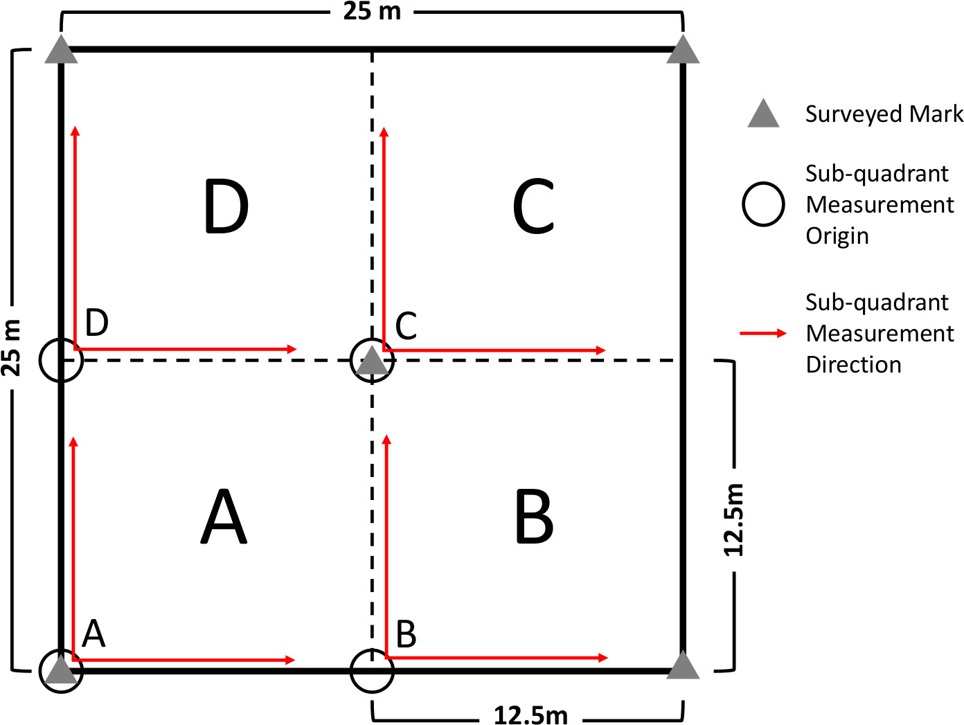
To facilitate stem census, in particular the estimation of stem XY location within 25 m × 25 m quadrats, total station surveying equipment was also used to identify the center point (centroid) of each quadrat. During census, field teams used the centroid to sub-divide each quadrat into 4 12.5 m × 12.5 sub-quadrants (Fig. 3). Trees were censused on a sub-quadrant basis for each quadrat. Census of all woody stems within each 25 m × 25 m quadrat was carried out by teams of three or four people. First, four 30 m long meter tapes are secured along each 25 m edge of the quadrat, drawn taught by attaching the tape to a stake; these tapes serve to delineate the entire 25 m × 25 m quadrat boundary. Then, for each sub-quadrant (A-D), the origin (0 m) of two more tapes are secured at the 'lower-left' corner of the sub-quadrant at right angles (circles in Fig. 3) and run along the 'lower' and 'left' edges of the sub-quadrant for a length of 12.5 m (red arrows in Fig. 3).

Due to constraints of prior field surveys, 25 m × 25 m quadrat grids at Knoll and Herbert Run were rotated relative to UTM grid north. 'Local' quadrat coordinates were recorded within each quadrat relative to the lower-left corner of the quadrat (point A in Fig. 3) and were transformed into 'global' UTM projected coordinates by first rotating the local coordinates relative to the UTM grid north and then translating relative to the UTM coordinates of the lower-left corner of the quadrat. The following rotation values in radians (θ) were used: Knoll = -0.012999 radians; Herbert Run = -0.676065 radians. Stem coordinates were therefore transformed from local coordinates ('lx' & 'ly') to global coordinates ('gx' & 'gy') by the following two equations:

gx = (lx×cosθ - ly×sinθ ) + qllX gy = (lx×sinθ + ly×cosθ ) + qllY
Where qllX and qllY refer to the X and Y coordinates of the lower left corner of the quadrat in meters UTM. Knoll and Herbert Run grid rotation (θ) parameters: Knoll = -0.012999 radiansHerbert Run = -0.676065 radians

Fig. 3: Diagram of 25 m × 25 m quadrat grid lay out with 12.5 m × 12.5 m census sub-quadrants and configuration of sub-quadrant measurement system.

3. Research Methods

Instrumentation:

A Sokkia SET 510a Total Station with Trimble TSC-2 Data Logger were used to lay out the 25 m × 25 m quadrat grid. Details of the surveying workflow can be found at the Ecosynth project website (http://wiki.ecosynth.org/index.php?title=Plot_Surveying_Protocol, accessed 2014/11/07). Positioning of quadrat grid points (gray triangles in Fig. 3) by total station was based off of local high-accuracy control points. Control points included existing brass geodetic monuments and additional markers positioned around the two census plots by survey traverse methods and by centimeter precision RTK-GPS mapping by UMBC Facilities personnel (real time kinematic - global positioning system). The 25 m × 25 m quadrat grid was created first in GIS then uploaded into the total station and points were located in the field by 'stake-out' method with estimated horizontal root mean square error of 0.2–0.3 m (RMSE) based on a resurvey of ≈ 30 points. An 8" (20.3 cm) galvanized steel nail, sunken into the ground marked each surveyed quadrat grid corner point and center point in forest and grass areas. For quadrat corners located on pavement, 1" (2.54 cm) steel survey nails were used to mark surveyed points.

After quadrats and sub-quadrants were marked with tapes, field teams tagged all woody stems ≥ 1 cm DBH using numbered aluminum tags. Tags were affixed with nails on trees ≥ 10 cm DBH and using loose metal wire for smaller stems. When a tag was placed on a stem, the DBH and tag number of the stem were recorded in the 'Main Data Sheet'. All stems across both sites are assigned an unique tag number, there are no duplicate tag numbers between Knoll and Herbert Run. The point of measurement of DBH measurements was identified by a wooden pole of length 1.37 m and DBH was measured on the up-hill side of a tree parallel to the trunk following Condit (1998). If DBH could not be measured at 1.37 m, diameter was measured at an alternate height as recorded in the HOM (height of measurement) field on the data sheet, otherwise HOM was 1.37 m. For trees with multiple stems that are separated below DBH, the tag was placed on the largest stem and the DBH of that stem was recorded on the 'Main Data Sheet'. DBH of other stems associated with that tag number were recorded on the 'Multiple Stem Sheet'. Special codes were used to characterize the stems as needed, including codes for multiple stems ('M'), dead stems ('D'), stems that are leaning or topped off, or other issues. Special stem codes are described in Section IV.B Variable Information.

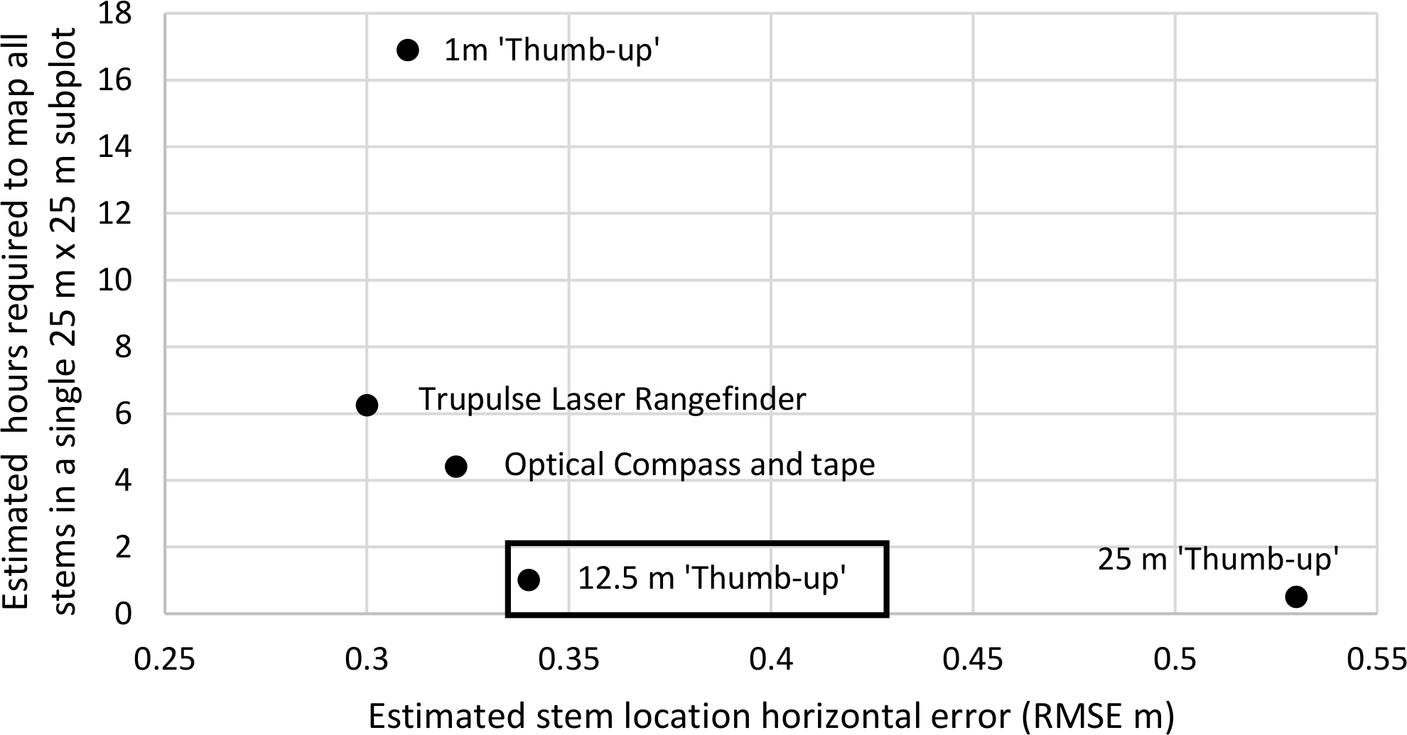
Stem locations were mapped by eye to determine the perpendicular distance of a tree from meter tapes placed orthogonally along the 'lower' (horizontal, X) and 'left' (vertical, Y) 12.5 m × 12.5 m sub-quadrant edges (Condit 1998). This method was referred to within the project as the '12.5 m thumb-up' method. Sub-quadrant code (A–D), X and Y distance are recorded on the 'Main Data Sheet' for each stem. This approach required roughly one hour per 25 m × 25 quadrat for teams of 3–4 and produced tree stem locations with roughly 0.34 m horizontal RMSE error compared to mapping stem location with the total station, which is expected to produce sub-centimeter precision measurements. Other approaches based on optical compass, laser rangefinder, or smaller subplot segmentations produced similar positioning accuracy with significantly increased labor cost (Fig. 5, Section V.C Related Material).

Data recorded for each stem on the 'Main Data Sheet' and 'Multiple Stem Sheet' was entered into an electronic spreadsheet for additional processing. Stem locations were transformed into geographic locations within the WGS84 (World Geodetic System 1984 datum) UTM Zone 18N projected coordinate system by first translating the measurements from sub-quadrant-based to quadrat-based ('lower-left', origin A, Fig. 3) by adding 12.5 m to either X or Y measurement (or both) as needed. Quadrat-based stem coordinates were then rotated to match the orientation of the entire quadrat grid relative to UTM grid north. Finally, stem locations were translated into the UTM coordinate system by addition of the corresponding UTM Northing (Y) and Easting (X) coordinates of the 'lower-left' corner of the subplot (point A, Figure 3). Refer to Section II.2 Permanent Plots for details about local to global stem coordinate transformations. For trees located outside of forested areas where it was not possible or practical to establish a 25 m × 25 m quadrat grid (e.g., planted and ornamental street trees; Fig. 2), location was recorded by precision RTK-GPS (sub-meter accuracy) or by photo interpretation of tree center from high-resolution aerial imagery (Baltimore County Office of Information Technology; 0.6 m horizontal accuracy, 0.3 m pixel resolution; collected 2008/03/01 – 2008/04/01).

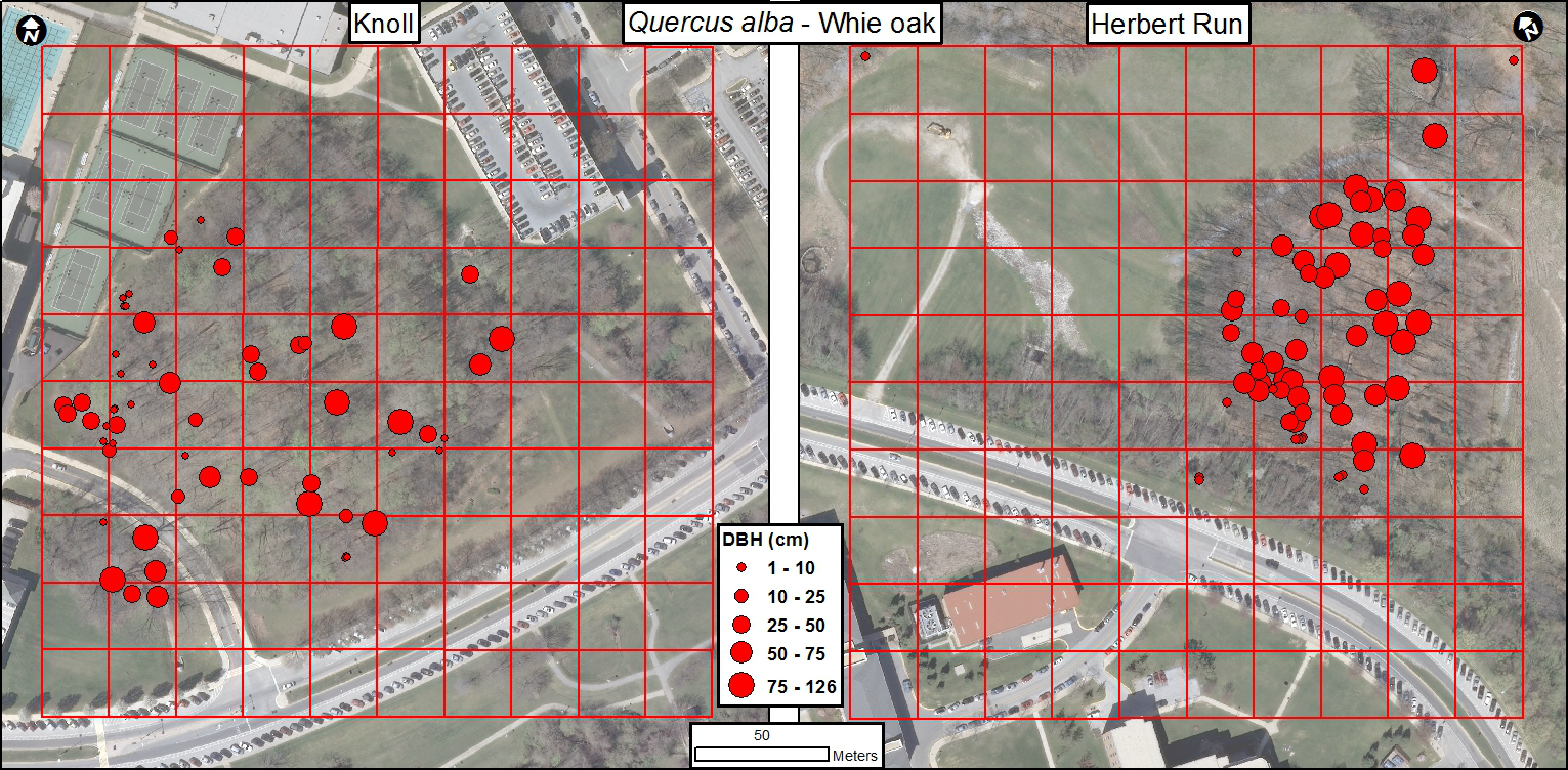
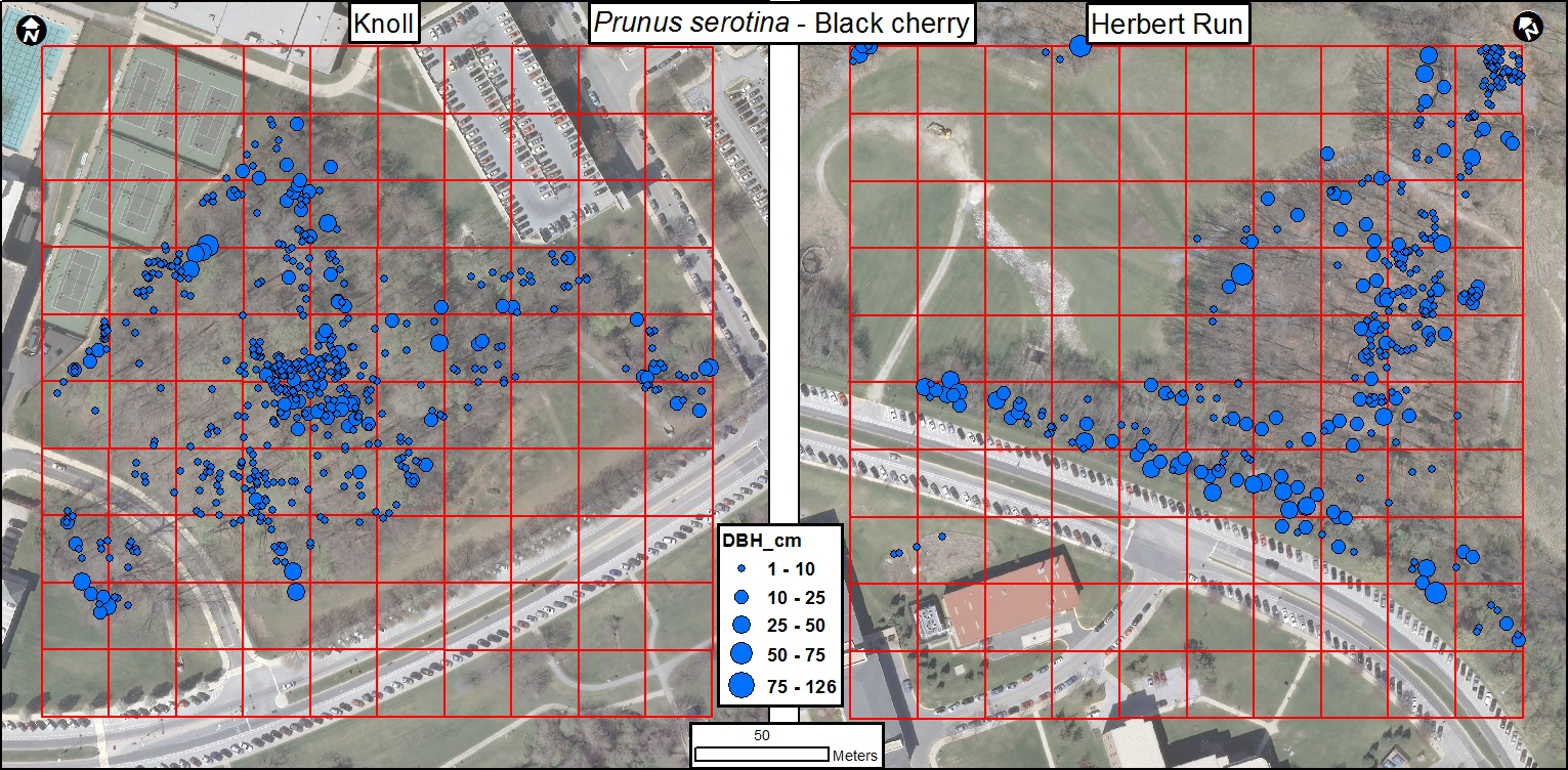
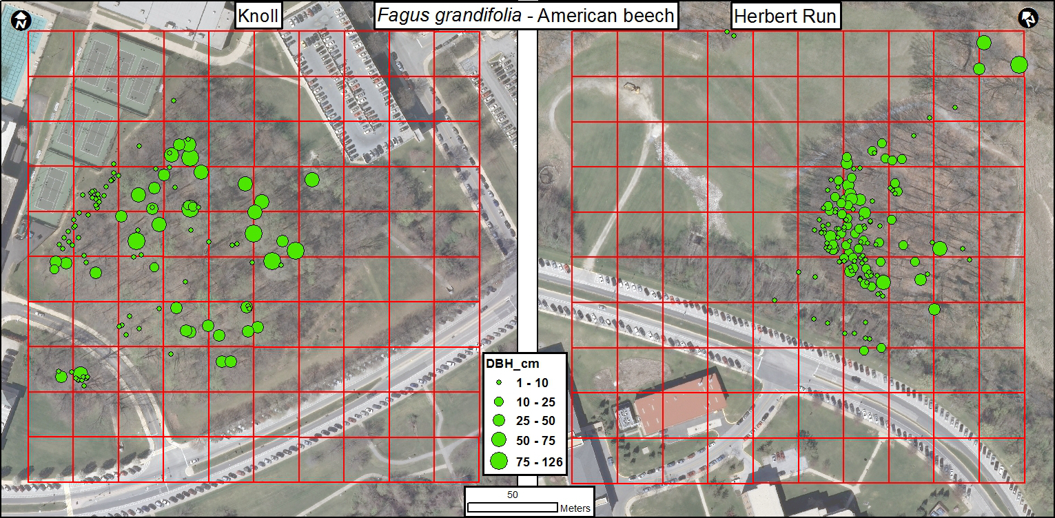
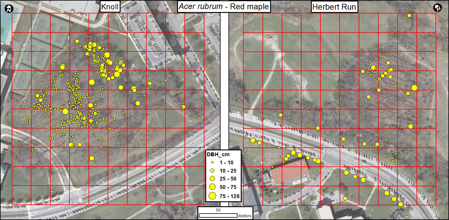
Taxonomy: Taxonomy of all living stems was carried out in three passes with three field workers. In the first pass, a student worker visited all stems and attempted to identify each stem to either genus or species with the highest degree of certainty. For example, if there was a large degree of evidence for the genus Fraxinus (Ash), but it was not possible to collect enough information to distinguish between the common species observed in the area, americana (White) or pennsylvanica (Green), then the stem was only identified to genus. Stems where there was not enough evidence to distinguish genus were marked as 'unknown'. In the second pass, the second worker visited those stems that were only identified to genus or were identified as 'unknown' by the first worker and using the same criteria attempted to identify stems to species. In the third and final pass, the third worker visited the stems left identified only to genus or as 'unknown' by the second worker and attempted to identify the remaining stems to species and group all unknown stems as unknown but of the same taxa. Taxonomy was not recorded for stems marked as dead. Table 2 shows the number of stems, basal area, and importance value of the top 25 taxa, ranked by importance value, defined as the sum of % basal area (dominance) and % density (Parker and Tibbs 2004). The primary taxonomy reference was the Audubon Society Field Guide to North American Trees along with several online references: Virginia Tech Dendrology Factsheets (http://dendro.cnre.vt.edu/dendrology/factsheets.cfm), and the USDA PLANTS Database (http://plants.usda.gov/java/). Supplemental maps in Fig. 4, Section V.C Related Material show the spatial distribution of five of the most dominant taxa (by importance value) at both plots.

Table 2: Total count, density, and basal area of all stems ≥ 1 cm DBH at Knoll and Herbert Run study sites combined (12.5 ha) of top 25 species sorted by importance value (IV), which comprised ≈ 90% of total stems and total basal area.
			Basal Area
Species	n	%	m2 ha-1	%	IV
Quercus alba	128	1.56	2.35	17.12	18.68
Prunus serotina	1060	12.94	0.69	5.05	17.99
Standing dead stemsa	856	10.45	0.80	5.84	16.29
Fagus grandifolia	338	4.12	1.05	7.68	11.80
Acer rubrum	631	7.70	0.49	3.54	11.24
Liriodendron tulipifera	81	0.99	1.23	8.96	9.95
Robinia pseudoacacia	302	3.69	0.80	5.80	9.49
Nyssa sylvatica	383	4.67	0.58	4.20	8.87
Fraxinus pennsylvanica	534	6.52	0.31	2.26	8.78
Quercus rubra	254	3.10	0.69	5.04	8.14
Acer saccharum	584	7.13	0.10	0.77	7.90
Carya cordiformis	418	5.10	0.23	1.66	6.76
Fraxinus americana	194	2.37	0.32	2.37	4.74
Acer negundo	230	2.81	0.25	1.85	4.66
Fraxinus sp.	88	1.07	0.48	3.53	4.60
Cornus florida	332	4.05	0.04	0.32	4.37
Quercus coccinea	48	0.59	0.47	3.42	4.01
Quercus phellos	46	0.56	0.47	3.41	3.97
Prunus avium	136	1.66	0.24	1.77	3.43
Quercus velutina	16	0.20	0.36	2.63	2.83
Sassafras albidum	190	2.32	0.07	0.51	2.83
Carya tomentosa	142	1.73	0.15	1.09	2.82
Carya glabra	137	1.67	0.15	1.11	2.78
Morus alba	124	1.51	0.14	0.99	2.50
Ulmus americana	97	1.18	0.15	1.12	2.30
49 othersb	845	10.32	1.09	7.94	18.26
Sums	8194	100	13.70	100	200
per hectare rate	656
a All free-standing stems ≥ 1 cm DBH that were ≥ 1.37 m tall.
b Refer to complete species list in UMBC_species_list_file.txt (Section IV.A Data Set File).

Permit history: All data collection done on UMBC property with the permission of University administration (Donna Andersen). No samples were collected or removed from plots.

Legal/organizational requirements: Site visits should be carried out with permission of project PIs Erle Ellis ([email protected]) and/or Matthew Baker (UMBC Associate Professor; [email protected]).

4. Project personnel: The project PI was Erle C. Ellis (NSF grant PI, Associate Professor). Other personnel directly involved in preparation of datasets and day-to-day field work: Jonathan P. Dandois (project initiation, plot selection, definition of measurement protocol, supervision of fieldwork and species identification, project supervision during length of project, overall data supervisor, and data publication lead author), Dana Nadwodny (day-to-day manager of field technicians and interns, manager of database and field data entry), Andrew Jablonski (methods documentation), Jaicy Ferguson and Ilan Segal (species ID), Erik Andersen (testing and accuracy assessment of measurement protocol and associated documentation), Andrew Bofto (sampling plot grid total station surveying and associated documentation), Shane McFaul (field technician, data entry, and database management), as well as the following field technicians that contributed to data collection and entry: Dana Boyd, Natalie Cheetoo, Maeve Tilly, Darryl Wise, Svetlana Peshkoff, Zachary Bergeron, Alexa White, Britany Warren, Kirsten McGovern, and Ryan Garvis. In addition, William Wiley (UMBC campus geospatial and survey control assistance), Geoffrey Parker and Joshua Brinks (SERC, advice in methods protocol development) provided invaluable assistance to the project. Erle Ellis and Matthew Baker are current project PIs at the time of initial preparation of the metadata.

Class III. Data set status and accessibility

A. Status

Latest update: August 2014.

Latest Archive date: August 2014.

Metadata status: The metadata are complete and up-to-date.

Data verification: Data quality was maintained through revisit and verification of field measurements when potentially erroneous records were observed in the tree stem location GIS file. Correction of erroneous records included changing tag numbers or location based on re-measurement. Taxonomic identification for stems that were suspect (a single taxa that is uncommon to the area) or to a coarser than species level (genus only) was verified by revisit in different seasons when it was possible to observe other identifying traits like leaves, fruits, flowers, or new twig buds.

B. Accessibility

Storage location and medium: Physical and digital scanned copies of the data sheets for the original census are stored in the Laboratory for Anthropogenic Landscape Ecology in the Department of Geography and Environmental Systems at UMBC, Sondheim Hall 002C. Digital data files are also stored within the database of the Smithsonian Institute ForestGeo network (http://www.forestgeo.si.edu/).

Contact person: Dr. Erle C. Ellis, Associate Professor, [email protected]

Copyright restrictions: Content is made available under CC BY 4.0.

Proprietary restrictions: None, the data are free to use for further analyses, with due citations to this data paper and, when appropriate, to Dandois and Ellis (2013).

Class IV. Data structural descriptors

A. Data Set File

Identity: Original and most current census are available through the SI ForestGeo network (http://www.forestgeo.si.edu/).

Size: The number of rows and columns includes headers; size is given for uncompressed files.

Format and storage mode: ASCII text, tab delimited.

Header information: Headers corresponding to variable names (see IV.B.Variable definitions) are included as first row in the data file.

Alphanumeric attributes: Mixed: upper and lower case.

Special characters/fields:No data values are left blank in census file. The species codes 'NOFND' and 'ZDEAD' are not actual taxonomic codes, but refer instead to trees that could not be found for ID after initial mapping 'NOFND' or which were identified only as dead, 'ZDEAD'. Values of 'N/A' in species list file refer to non-applicable entries.

Au

^a MD5 checksum values computed in R version 3.1.1 using the function "md5sum" in the standard library "tools" (R Core Team 2014).

B. Variable information

Variable names are headers included as first row in the data file. All data is formatted following Handbook for management of CTFS databases.

Data anomalies: There are no known data anomalies.

Class V. Supplemental descriptors

A. Data acquisition

A. Data acquisition

Data forms: All original field census data were recorded on empty data sheets following Condit 1998. Field data sheets required field technicians to enter the site (KN or HR) the quadrat number, (1-100), the sub-quadrant letter (A-D), and the date of census. For each stem, technicians recorded the: tag number, DBH, the X and Y coordinates of the location of the stem within the sub-quadrant, and any special codes for that stem. For trees with multiple stems, the special code 'M' was indicated for a stem on the 'Main Data Sheet' and the DBH of all other stems of that tree were recorded on the 'Multiple Stem Sheet' along with the tag number for that tree. Using the same forms and after data entry into electronic spreadsheet and GIS, taxonomic survey teams then revisited each stem and indicated the genus and species of the stem.

Location of completed data forms:Physical and digital scanned copies of the data sheets for the original census are stored in the Laboratory for Anthropogenic Landscape Ecology in the Department of Geography and Environmental Systems at UMBC, Sondheim Hall 002C.

Data entry/verification procedures: Field census data were first transferred from field data forms into an electronic spreadsheet by a field technician on the day of or the day after data collection. After data entry, forms were digitized by scanner and stored in electronic archives. Data entry quality was confirmed by data manager by looking for any anomalous entries, for example: wrong columns, skipped columns, numbers out of range for a DBH or sub-quadrant x and y due to transposition of columns at time of field or electronic entry. Errors in field data entry at this stage were corrected by reviewing the scanned data forms or by re-visit to plot as needed.

B. Quality assurance/quality control procedures: Data quality was assessed when tree stem locations were transformed into GIS, at which time errors in field entry of stem locations became apparent: trees in wrong 25 m quadrat or 12.5 m sub-quadrant. Errors were corrected by review of field data sheets or by new field visit to re-measure as needed. Additional errors (wrong tag number, missing tag number, wrong location, missing tree stem) that were identified during additional visits, for example during taxonomic survey, were similarly corrected by re-measurement in the field. Finally, data quality was assessed by analysis of entire database of records: duplicate tag numbers for stems of different species / in different plots, trees in the wrong location. These errors were also addressed by revisit to stems and updating of electronic database.

C. Related material:

Figure 4: Stem maps of the top 5 most common species across both plots, as determined by importance value (IV, Table 2). Stem location points are shown with a relative scale based on classes of stem diameter (DBH) but for visual clarity do not reflect true diameter relative to the map scale. Image source: see Fig. 1. Image shown with 30 % transparency to enhance visual clarity of stem points.

Figure 5: Comparison of the difference in stem location positioning accuracy for different methods as a function of the time required to map an entire 25 m × 25 m plot. The accuracy of stem locations was computed as meters RMSE (root mean square error) against locations measured via total station surveying which served as 'ground-truth' (estimated precision = 0.03 m). '12.5 m Thumb-up' was selected for providing optimal balance of time and error.

Description of methods: 1 m 'Thumb-up', perpendicular distance to two orthogonal tapes within a 1 m × 1 m sub-quadrant grid; Trupulse Laser Rangefinder, location estimated by distance and bearing from quadrat origin based on using rangefinder distance and azimuth functions; Optical compass and tape, location estimated by distance and bearing from quadrat origin from optical (analog) compass and meter tape; 12.5 m 'Thumb-up', perpendicular distance to two orthogonal tapes along lower and left edges of 12.5 m × 12.5 m sub-quadrant grid; 25 m 'Thumb-up', perpendicular distance to two orthogonal tapes along lower and left edges of entire 25 m × 25 m quadrat.

D. Computer programs and data processing algorithms: Refer to Section II.2 Permanent Plots for details about the two-dimensional rotation algorithm applied to transform coordinates from the local reference to the UTM global reference.

E. Archiving: Original field data sheets are stored as electronic and paper copies at the UMBC lab, refer to Section III.B Accessibility for details. Digital data files are also stored within the database of the Smithsonian Institute ForestGeo network (http://www.forestgeo.si.edu/).

F. Publication and results: Dandois and Ellis 2013.

G. History of data set usage:

Data set update history: Updated versions of the dataset based on planned 5-year re-census will be available from the Smithsonian Institute ForestGeo network (http://www.forestgeo.si.edu/).

Literature cited

Anderson-Teixeira, K. J., S. J. Davies, A. C. Bennett, E. B. Gonzalez-Akre, H. C. Muller-Landau, S. Joseph Wright, K. Abu Salim, A. M. Almeyda Zambrano, A. Alonso, J. L. Baltzer, Y. Basset, N. A. Bourg, E. N. Broadbent, W. Y. Brockelman, S. Bunyavejchewin, D. F. R. P. Burslem, N. Butt, M. Cao, D. Cardenas, G. B. Chuyong, K. Clay, S. Cordell, H. S. Dattaraja, X. Deng, M. Detto, X. Du, A. Duque, D. L. Erikson, C. E. N. Ewango, G. A. Fischer, C. Fletcher, R. B. Foster, C. P. Giardina, G. S. Gilbert, N. Gunatilleke, S. Gunatilleke, Z. Hao, W. W. Hargrove, T. B. Hart, B. C. H. Hau, F. He, F. M. Hoffman, R. W. Howe, S. P. Hubbell, F. M. Inman-Narahari, P. A. Jansen, M. Jiang, D. J. Johnson, M. Kanzaki, A. R. Kassim, D. Kenfack, S. Kibet, S., M. F. Kinnaird, L. Korte, K. Kral, J. Kumar, A. J. Larson, Y. Li, X. Li, S. Liu, S. K. Y. Lum, J. A. Lutz, K. Ma, D. M. Maddalena, J. -R. Makana, Y. Malhi, T. Marthews, R. Mat Serudin, S. M. McMahon, W. J. McShea, H. R. Memiaghe, X. Mi, T. Mizuno, M. Morecroft, J. A. Myers, V. Novotny, A. A. de Oliveira, P. S. Ong, D. A. Orwig, R. Ostertag, J. den Ouden, G. G. Parker, R. P. Phillips, L. Sack, M. N. Sainge, W. Sang, K. Sri-ngernyuang, P. R. Sukumar, I. F. Sun, W. Sungpalee, H. S. Suresh, S. Tan, S. C. Thomas, D. W. Thomas, J. Thompson, B. L. Turner, M. Uriarte, R. Valencia, M. I. Vallejo, A. Vicentini, T. VrÅ¡ka, X. Wang, X. Wang, G. Weiblen, A. Wolf, H. Xu, S. Yap, and J. Zimmerman. 2014. CTFS-ForestGEO: a worldwide network monitoring forests in an era of global change. Global Change Biology 21:528–549.

Bolund, P., and S. Hunhammar. 1999. Ecosystem services in urban areas. Ecological Economics 29:293–301.

Brush, G.S., C. Lenk, and J. Smith. 1980. The natural forests of Maryland: An explanation of the vegetation map of Maryland. Ecological Monographs, 50(1):77–92.

Cadenasso, M. L., and S. T. A. Pickett. 2001. Effect of Edge Structure on the Flux of Species into Forest Interiors. Conservation Biology 15:91–97.

Condit, R. 1998. Tropical forest census plots. Berlin: Springer.

Costanza, R., R. d'Arge, R. de Groot, S. Farber, M. Grasso, B. Hannon, K. Limburg, S. Naeem, R. V. O'Neill, J. Paruelo, R. G. Raskin, P. Sutton, and M. van den Belt. 1998. The value of the world's ecosystem services and natural capital. Ecological Economics 25:3–15.

Dandois, J. P., and E. C. Ellis. 2010. Remote sensing of vegetation structure using computer vision. Remote Sensing 2:1157–1176.

Dandois, J. P., and E. C. Ellis. 2013. High spatial resolution three-dimensional mapping of vegetation spectral dynamics using computer vision. Remote Sensing of Environment 136:259–276.

DeFries, R., F. Achard, S. Brown, M. Herold, D. Murdiyarso, B. Schlamadinger, and C. de Souza Jr, C. 2007. Earth observations for estimating greenhouse gas emissions from deforestation in developing countries. Environmental Science and Policy 10:385–394.

Dubayah, R.O., S. L. Sheldon, D. B. Clark, M. A. Hofton, J. B. Blair, G. C. Hurtt, and R. L. Chazdon. 2010. Estimation of tropical forest height and biomass dynamics using lidar remote sensing at La Selva, Costa Rica. Journal of Geophysical Research 115:G00E09.

Dwyer, J., McPherson, E., Schroeder, H., and Rowntree, R. 1992. Assessing the benefits and costs of the urban forest. Journal of Arboriculture 18:227–227.

Ellis, E. C., and N. Ramankutty. 2008. Putting people in the map: anthropogenic biomes of the world. Frontiers in Ecology and the Environment 6:439–447

FAO and JRC. 2012. Global forest land-use change 1990–2005, by E. J. Lindquist, R. D'Annunzio, A. Gerrand, K. MacDicken, F. Achard, R. Beuchle, A. Brink, H.D. Eva, P. Mayaux, J. San-Miguel-Ayanz and H-J. Stibig. In FAO Forestry Paper No. 169. Food and Agriculture Organization of the United Nations and European Commission Joint Research Centre. Rome, FAO.

Foley, J. A., R. DeFries, G. P. Asner, C. Barford, G. Bonan, S. R. Carpenter, F. S. Chapin, M. T. Coe, G. C. Daily, H. K. Gibbs, J. H. Helkowski, T. Holloway, E. A. Howard, C. J. Kucharik, C. Monfreda, J. A, Patz, I. C. Prentice, N. Ramankutty, and P. K. Snyder. 2005. Global Consequences of Land Use. Science 309:570–574.

Frolking, S., M. W. Palace, D. B. Clark, J. Q. Chambers, H. H. Shugart, and G. C. Hurtt. 2009. Forest disturbance and recovery: A general review in the context of spaceborne remote sensing of impacts on aboveground biomass and canopy structure. Journal of Geophysical Research 114.

Goetz, S., and R. Dubayah. 2011. Advances in remote sensing technology and implications for measuring and monitoring forest carbon stocks and change. Carbon Management 2:231–244.

Hobbs, E. R. 1988. Species richness of urban forest patches and implications for urban landscape diversity. Landscape Ecology 1:141–152.

Houghton, R. A., F. Hall, and S. J. Goetz. 2009. Importance of biomass in the global carbon cycle. Journal of Geophysical Research 114.

Lenth, B. A., R. L. Knight, and W. C. Gilgert. 2006. Conservation Value of Clustered Housing Developments. Conservation Biology 20:1445–1456.

Loyd, K. A. T., S. M. Hernandez, J. P. Carroll, K. J. Abernathy, and G. J. Marshall. 2013. Quantifying free-roaming domestic cat predation using animal-borne video cameras. Biological Conservation 160:183–189.

McPherson, E. G., D. Nowak, G. Heisler, S. Grimmond, C. Souch, R. Grant, and R. Rowntree. 1997. Quantifying urban forest structure, function, and value: the Chicago Urban Forest Climate Project. Urban Ecosystems 1:49–61.

Parker, G. G., and D. J. Tibbs. 2004. Structural phenology of the leaf community in the canopy of a Liriodendron tulipifera L. forest in Maryland, USA. Forest Science 50:387–397.

Pickett, S. T. A., M. L. Cadenasso, J. M. Grove, C. H. Nilon, R. V. Pouyat, W. C. Zipperer, and R. Costanza. 2001. Urban Ecological Systems: Linking Terrestrial Ecological, Physical, And Socioeconomic Components Of Metropolitan Areas. Annual Review of Ecology and Systematics 32:127.

Potere, D., A. Schneider, S. Angel, and D. L. Civco. 2009. Mapping urban areas on a global scale: which of the eight maps now available is more accurate? International Journal of Remote Sensing 30:6531–6558.

R Core Team. 2014. R: A language and environment for statistical computing. R Foundation for Statistical Computing, Vienna, Austria. URL http://www.R-project.org/.

Riitters, K., J. Wickham, R. O'Neill, B. Jones, and E. Smith. 2000. Global-scale patterns of forest fragmentation. Conservation Ecology 4.

Riitters, K. H., J. D. Wickham, R. V. O'Neill, K. B. Jones, E. R. Smith, J. W. Coulston, T. G. Wade, and J. H. Smith. 2002. Fragmentation of Continental United States Forests. Ecosystems 5:0815–0822.

Schimel, D., M. Keller, S. Berukoff, B. Kao, H. Loescher, H. Powell, T. Kampe, D. Moore, and W. Gram. 2011. NEON Science Infrastructure. In, NEON 2011 Science Strategy (pp. 36–38).

Turner, W. 2014. Sensing biodiversity. Science 346:301–302.

Vidra, R. L., T. H. Shear, and T. R. Wentworth. 2006. Testing the Paradigms of Exotic Species Invasion in Urban Riparian Forests. Natural Areas Journal 26:339–350.

[Back to E096-156]