Ecological Archives E096-122-A1
Meryl C. Mims, Ivan C. Phillipsen, David A. Lytle, Emily E. Hartfield Kirk, and Julian D. Olden. 2015. Ecological strategies predict associations between aquatic and genetic connectivity for dryland amphibians. Ecology 96:13711382. http://dx.doi.org/10.1890/14-0490.1
Appendix A. Description of sampling and genetic methods as well as assessment of potential bias due to different sampling methods. Appendix A also includes sampling maps for all three species and tables describing sampling and genetic information by site and by species, microsatellite loci for red-spotted toads and canyon treefrogs, results from Hardy Weinberg exact tests, microsatellite loci characteristics, STRUCTURE results, and results of assessment of bias across sampling methods.
Amphibian sampling
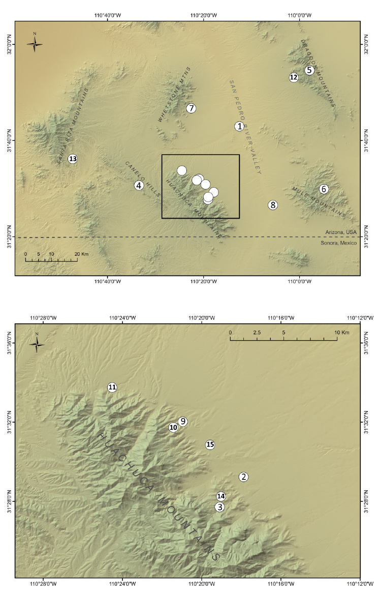
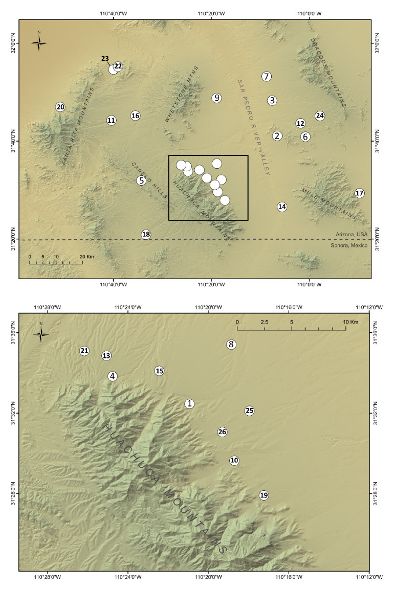
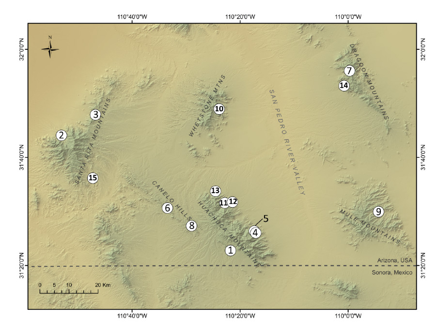
Sample sites for each species are shown in Fig. A1, A2, and A3, and sample-specific information is summarized by location in Table A1. Adults were collected at breeding sites and along roadways, and larval samples were collected with dip nets from breeding ponds. Where possible, multiple spatial or temporal replicates from a given sampling locale were collected (described in the main text). These temporal and spatial replicates ("Reps") were tallied and are presented in Table A1, and the genetic implications of variability in the number of replicates are discussed later in this appendix.
Microsatellite amplification and screening
Whole genomic DNA extractions were performed using DNeasy 96 Blood & Tissue Kit (QIAGEN), and extractions were performed at the Molecular Ecology Research Lab at the University of Washington's School of Aquatic and Fishery Sciences. Mexican spadefoot loci were compiled from previously published microsatellite markers (Rice et al. 2008, Van Den Bussche et al. 2009). Canyon treefrog and red-spotted toad marker sets were developed by the Evolutionary Genetics Core Facility at Cornell University and are described in Table A2. Polymerase chain reaction (PCR) was used to amplify DNA for multiplexed loci using Multiplex PCR kits (QIAGEN). PCR products were genotyped using an ABI 3730 sequencer (Applied Biosystems) at the Oregon State University's Center for Genome Research and Biocomputing (Corvallis, OR). Genotypes were analyzed using the software GENEMAPPER 4.1 (Applied Biosystems), and alleles were binned using the program TANDEM (Matschiner and Salzburger, 2009). Loci were screened for the presence of linkage disequilibrium using the log likelihood ratio statistic for each pair of loci in each population was found (GenePop, Raymond and Rousset 1995). No evidence of consistent linkage between loci was found. Any significant pairwise linkage results occurred in < 13% of all populations for a given species; results not shown but available upon request. Loci were also screened for deviations from Hardy-Weinberg equilibrium (HWE) using the exact p-test (results presented in Table A3) as implemented in GenePop (Raymond and Rousset 1995), and the presence of null alleles was evaluated with Micro-Checker (Van Oosterhout et al. 2004) using adults only (spadefoots) or larval samples from which all but one full sibling were removed. With a Bonferroni correction applied, no significant deviations from HWE were observed for any locus in a given population for canyon treefrogs or Mexican spadefoots. Three significant deviations from HWE were observed for red-spotted toads (Table A3); however, because these deviations did not represent a considerable proportion of tests for any given population or locus, all markers and populations were retained in our analyses. Summary statistics for all retained loci (all species) are included in Table A4, including F statistics calculated using MSA 4.05 (Dieringer and Schlötterer 2003).
Larval samples can bias population genetics findings by artificially inflating genetic differentiation due to family structure (Goldberg and Waits 2010); therefore, we screened all larval samples for full siblings using the program COLONY (Wang 2009). One sibling was retained from each family with fewer than six siblings. For families with six or more full siblings, there is a 98.4% chance of detecting both parental alleles for each locus, and we manually reconstructed two parental genotypes for use in population-based analyses for samples < 25 in order to achieve the maximum sample size. For individual-based analyses, only a single sibling was retained. This was confirmed by re-genotyping rare alleles (in < 3 individuals). We estimated statistical power of our final marker sets using POWSIM, a simulation-based computer program that estimates power (and α error) for chi-square and Fisher's exact tests when evaluating the hypothesis of genetic homogeneity (Ryman and Palm 2006). Sample sizes, number of samples, loci and allelic information, and number of generations can be combined under various scenarios to produce a hypothetical degree of genetic differentiation (measured as FST). We ran simulations for each species and used our actual sample size and number of samples (conservatively calculated without reconstructed parents), our median estimated Ne, numbers of loci and alleles, and allele frequency for simulations. Number of generations was then adjusted to approximate observed FST. Each species was simulated at a range of numbers of generations from 10 to 500 to calculate power at a range of FST output values, including one that approximated the observed FST. Proportion of significant differences observed (200 runs) was 1.0 for all species in almost all scenarios. The 10-generation spadefoot simulations were the only scenario with a proportion of significant differences observed that fell below 1.0. However, the estimated FST for that run was roughly 1/10 the observed FST, indicating that a 10-generation simulation is not sufficiently long to reflect actual observed genetic differentiation for this species. These results indicate satisfactory statistical power given the loci and sample sizes in our data set.
Hierarchical population structure and clustering
Individual-based hierarchical population structure was analyzed using the Bayesian clustering program STRUCTURE 2.3.4 (Pritchard et al. 2000). Each sampling site was treated as an independent putative population with a total of n putative populations for each species. Ten iterations of each K from 1 to n + 1 for each species were run for 1,000,000 cycles with a burn-in of 200,000 cycles. We used the locprior model with admixture and correlated allele frequencies. The most likely K was determined using the delta-K method (Evanno et al. 2005) in which the most likely value of K is assessed by the second-order rate of change in the log-likelihood. A delta-K value cannot be calculated for K = 1; thus, for cases in which K = 1 has the greatest log-likelihood, 1 is assumed to be the most likely K (Spear et al. 2012). This analysis was repeated for genetic clusters in which both K > 1 and n > 1 to identify hierarchical population structure until terminal clusters were described (Phillipsen et al. 2013). All STRUCTURE output and delta-K calculations are included in Table A5. STRUCTURE output was visualized using the program DISTRUCT 1.1 (Rosenberg 2004).
Assessment of potential sampling bias from variable sampling methods
Despite accounting for larval family structure, it is possible that variable sampling methods may introduce biases into genetic inference of population structure and connectivity. For example, COLONY accounts for full-sibling groups, but it is possible that half-siblings or other distant family structure inflates genetic differentiation between larval samples relative to adult samples. Also, Mexican spadefoot adults were collected along roadways in addition to breeding sites. It is not well known whether adults of this species exhibit breeding site fidelity or homing behavior; if they do, particularly for their larval pond, it is reasonable to expect that adults collected at breeding sites may be more genetically similar than those collected along roads. To examine whether we see evidence of large bias from these variable sampling methods, we paired larval samples with nearby adult samples for red-spotted toads and spadefoots. Canyon treefrogs were not included because we did not have enough adult samples to generate a sufficient number of adult-larval paired samples. We then examined genetic diversity and overall genetic differentiation within each group of samples collected by a given method (larval samples, adult samples, breeding site adults, and roadside adults).
Allelic richness and heterozygosity were similar across sampling methods within species. We found some evidence for higher differentiation among larval samples than adult samples for red-spotted toads, where G'ST increased by 62% for larval samples compared to adult samples (Table A6). Ne was also lower for larval samples than adults. However, for spadefoots, there was modest evidence of lower genetic differentiation among larval samples than for adult samples, with G'ST reduced by 34% for larval samples compared to adult samples. Ne was also lower for adult samples than for larvae for which the median Ne value was 10,000 (the estimate for infinite population sizes). Genetic differentiation between spadefoot adult sampling methods was minimal. However, for both species, not all "pairs" of larval and adult samples were spatially congruent. Some adult and larval red-spotted toad pairs were selected based on similar sample sizes and similar spatial locations, but with local processes identified as important for this species (for example, low Ne in some populations), the pattern of higher G'ST may be spurious and requires further exploration.
We also explored the effects of multiple sampling replicates ("Reps") in space and time on genetic diversity indices. To do this, we used a paired sample approach for populations of all three species with two or more replicates (from which at least 10 % of the sampled individuals represented an additional replicate). These included 3 populations of canyon treefrogs, 6 populations of red-spotted toads, and 12 populations of spadefoots. Due to low sample sizes for two of the three species, we did not explore effects of sampling replicates on genetic differentiation between populations. Genetic diversity metrics (HO, HE, AR, Ne and the upper confidence limit of Ne (Ne high) calculated using a jackknifing approach and estimated as 10,000 for infinite values) were calculated with only one replicate and with multiple replicates. To control for sample size, multiple replicate samples were reduced to match sample sizes of one replicate only. Where possible, equal numbers of individuals were included from each replicate in the reduced sample. A paired t-test was then used to compare differences in HO, HE and AR, and a Wilcoxon signed-rank test was used to compare differences in Ne and the upper confidence interval of Ne given the non-normal distribution of differences for these values. Local processes such as drift due to low Ne or low migration rates as well as possible metapopulation dynamics were identified as playing a greater role in population genetic structure of canyon treefrogs and red-spotted toads, and the effect of multiple sampling replicates may be more apparent in species such as these with low Ne and greater family structure among larval samples. For that reason, the effect of replicates on these genetic diversity metrics was calculated for all species as well as for canyon treefrogs and red-spotted toads combined.
We found little evidence that sample replicates biased the results of this study (Table A7). We found no significant differences in genetic diversity measures between single and replicate samples for all species, and we found only one significant difference for canyon treefrog and red-spotted toads alone (HE, p value = 0.024). If a Bonferroni correction for multiple comparisons is applied, the result for HE is not significant.
In summary, although we saw differences in estimates of genetic differentiation between larval and adult samples for both species, the range of G'ST values within species were comparatively low. These potential biases did not result in overlap of G'ST between species, and thus for this study we suspect that the potential bias did not affect the outcome of this study. We also found little support for the effect of number of spatial or temporal sampling replicates on the genetic diversity metrics of this study. However, our results are limited to our study species in a subsection of their ranges, and bias due to different sampling methods may be more substantial for other species or regions. Future consideration of biases from sampling methods both in empirical and simulation studies may be particularly important for development of predictive models in which small differences in connectivity estimates may have implications for resistance surface parameterization or management actions.
Literature cited
Bowcock, A. M., A. Ruiz-Linares, J. Tomfohrde, E. Minch, J. R. Kidd, and L. L. Cavalli-Sforza. 1994. High resolution human evolutionary trees with polymorphic microsatellites. Nature 368:455–457.
Dieringer, D., and C. Schlötterer. 2003. Microsatellite analyser (MSA): a platform independent analysis tool for large microsatellite data sets. Molecular Ecology Notes 3:167–169.
Evanno, G., S. Regnaut, and J. Goudet. 2005. Detecting the number of clusters of individuals using the software STRUCTURE: a simulation study. Molecular Ecology 14:2611–2620.
Goldberg, C. S., and L. P. Waits. 2010. Quantification and reduction of bias from sampling larvae to infer population and landscape genetic structure. Molecular Ecology Resources 10:304–313.
Matschiner, M., and W. Salzburger. 2009. TANDEM: integrating automated allele binning into genetics and genomics workflows. Bioinformatics 25:1982–1983.
Phillipsen, I. C., and D. A. Lytle. 2013. Aquatic insects in a sea of desert: population genetic structure is shaped by limited dispersal in a naturally fragmented landscape. Ecography 36:731–743.
Pritchard, J. K., M. Stephens, and P. Donnelly. 2000. Inference of population structure using multilocus genotype data. Genetics 155:945–959.
Raymond, M., and F. Rousset. 1995. GENEPOP (version 1.2): population genetics software for exact tests and ecumenicism. Journal of Heredity 86:248–249.
Rice, A. M., D. E. Pearse, T. Becker, R. A. Newman, C. Lebonville, G. R. Harper, and K. S. Pfennig. 2008. Development and characterization of nine polymorphic microsatellite markers for Mexican spadefoot toads (Spea multiplicata) with cross-amplification in plains spadefoot toads (S. bombifrons). Molecular Ecology Resources 8:1386–1389.
Rosenberg, N. A. 2004. Distruct: a program for the graphical display of population structure. Molecular Ecology Notes 4:137–138.
Ryman, N., and S. Palm. 2006. POWSIM: a computer program for assessing statistical power when testing for genetic differentiation. Molecular Ecology 6:600–602.
Spear, S. F., C. M. Crisafulli, and A. Storfer. 2012. Genetic structure among coastal tailed frog populations at Mount St. Helens is moderated by post-disturbance management. Ecological Applications 22:856–869.
Van Den Bussche, R. A., J. B. Lack, C. E. Stanley, J. E. Wilkinson, P. S. Truman, L. M. Smith, and S. T. McMurry. 2009. Development and characterization of 10 polymorphic tetranucleotide microsatellite markers for New Mexico spadefoot toads (Spea multiplicata). Conservation Genetics Resources 1:71–73.
Van Oosterhout, C., W. F. Hutchinson, D. P. M. Wills, and P. Shipley. 2004. MICRO-CHECKER: software for identifying and correcting genotyping errors in microsatellite data. Molecular Ecology Notes 4:535–538.
Wang, I. J. 2009. A new method for estimating effective population sizes from a single sample of multilocus genotypes. Molecular Ecology 18:2148–2164.
Fig. A1. Canyon treefrog sampling map.
Fig. A2. Red-spotted toad sampling map.
Fig. A3. Mexican spadefoot sampling map.
Table A1. Sample number and locations (UTM Zone 12); sample size with siblings removed (N All), with reconstructed parents (N with P), and with number and percent of adults; replicates (temporal or spatial); allelic richness (based on minimum sample size); expected and observed heterozygosity; effective population size (Ne) and the 95% confidence intervals for Ne calculated via a jackknifing method where "Inf" represents infinity; and FIS values averaged over all loci. Results from Hardy Weinberg exact tests are included in Table A3. Additional information by locus and/or population are available from M.C. Mims upon request.
| Canyon treefrog | ||||||||||||||
Site |
UTM |
UTM |
N |
N |
N |
Percent Adults |
Reps |
AR |
HE |
HO |
Ne |
C.I.s for Ne |
FIS |
|
1 |
560558 |
3471841 |
19 |
19 |
15 |
79 |
1 |
4.96 |
0.71 |
0.75 |
17.9 |
12.7 |
27.4 |
-0.07 |
2 |
510906 |
3511050 |
10 |
11 |
2 |
20 |
1 |
6.45 |
0.81 |
0.84 |
Inf |
52.2 |
Inf |
-0.06 |
3 |
520834 |
3518105 |
7 |
8 |
2 |
29 |
2 |
5.26 |
0.78 |
0.81 |
13.5 |
8.7 |
24.4 |
-0.09 |
4 |
567504 |
3478529 |
7 |
11 |
0 |
0 |
1 |
4.58 |
0.71 |
0.73 |
7.5 |
3.1 |
16.2 |
-0.05 |
5 |
567930 |
3477919 |
8 |
10 |
0 |
0 |
1 |
4.66 |
0.74 |
0.78 |
7.4 |
3.7 |
13.4 |
-0.09 |
6 |
541988 |
3486290 |
5 |
7 |
0 |
0 |
1 |
5.50 |
0.72 |
0.68 |
Inf |
26.2 |
Inf |
0.08 |
7 |
594936 |
3533556 |
12 |
12 |
4 |
33 |
1 |
4.53 |
0.63 |
0.58 |
17.6 |
8.7 |
64.2 |
0.09 |
8 |
549066 |
3480211 |
10 |
12 |
3 |
30 |
2 |
5.65 |
0.79 |
0.81 |
33.1 |
15.5 |
348 |
-0.05 |
9 |
603435 |
3485393 |
9 |
13 |
1 |
11 |
2 |
3.06 |
0.54 |
0.54 |
2.7 |
1.8 |
6.7 |
-0.02 |
10 |
556976 |
3520186 |
15 |
16 |
0 |
0 |
1 |
4.33 |
0.70 |
0.74 |
Inf |
75.7 |
Inf |
-0.08 |
11 |
558781 |
3488127 |
17 |
17 |
17 |
100 |
1 |
5.54 |
0.80 |
0.81 |
30.7 |
18.7 |
67.5 |
-0.02 |
12 |
561038 |
3488403 |
22 |
23 |
0 |
0 |
2 |
5.62 |
0.79 |
0.75 |
323.1 |
72.3 |
Inf |
0.04 |
13 |
556064 |
3492110 |
6 |
9 |
0 |
0 |
1 |
5.79 |
0.79 |
0.84 |
75.1 |
25.9 |
Inf |
-0.11 |
14 |
593398 |
3528429 |
9 |
12 |
0 |
0 |
1 |
4.35 |
0.64 |
0.60 |
19.7 |
9.6 |
83.5 |
0.04 |
15 |
520105 |
3496453 |
19 |
22 |
0 |
0 |
1 |
6.05 |
0.80 |
0.83 |
94.4 |
35.1 |
Inf |
-0.05 |
Table A1, continued. |
||||||||||||||
Red-spotted toad |
||||||||||||||
Site |
UTM |
UTM |
N |
N |
N |
Percent Adults |
Reps |
AR |
HE |
HO |
Ne |
C.I.s for Ne |
FIS |
|
1 |
574944 |
3509235 |
11 |
12 |
0 |
0 |
2 |
3.88 |
0.65 |
0.69 |
6.9 |
3.3 |
11.7 |
-0.09 |
2 |
566670 |
3483820 |
8 |
8 |
0 |
0 |
1 |
5.81 |
0.83 |
0.78 |
Inf |
287.2 |
Inf |
0.03 |
3 |
564771 |
3481006 |
15 |
15 |
0 |
0 |
1 |
5.55 |
0.79 |
0.75 |
302.1 |
49.1 |
Inf |
0.05 |
4 |
542015 |
3486332 |
17 |
18 |
0 |
0 |
3 |
5.05 |
0.76 |
0.70 |
20 |
14.4 |
30.1 |
0.07 |
5 |
597845 |
3530951 |
9 |
11 |
0 |
0 |
1 |
5.99 |
0.80 |
0.82 |
Inf |
49.9 |
Inf |
-0.05 |
6 |
603007 |
3485338 |
9 |
11 |
0 |
0 |
2 |
4.36 |
0.67 |
0.68 |
2.9 |
2.3 |
4.9 |
-0.03 |
7 |
559054 |
3516045 |
6 |
9 |
0 |
0 |
1 |
5.28 |
0.77 |
0.73 |
Inf |
180.6 |
Inf |
0.02 |
8 |
586216 |
3479036 |
13 |
13 |
13 |
100 |
1 |
5.08 |
0.75 |
0.76 |
7.8 |
5 |
11.8 |
-0.04 |
9 |
561774 |
3488938 |
22 |
24 |
17 |
77 |
3 |
4.87 |
0.72 |
0.67 |
37.6 |
25.2 |
65.8 |
0.06 |
10 |
561034 |
3488404 |
6 |
6 |
0 |
0 |
1 |
5.93 |
0.79 |
0.72 |
Inf |
Inf |
Inf |
0.05 |
11 |
556119 |
3492102 |
48 |
48 |
25 |
52 |
5 |
5.61 |
0.80 |
0.82 |
46.4 |
37.7 |
58.5 |
-0.04 |
12 |
592703 |
3528123 |
10 |
15 |
0 |
0 |
1 |
5.52 |
0.76 |
0.74 |
83 |
37.2 |
Inf |
0.00 |
13 |
520105 |
3496453 |
17 |
18 |
2 |
12 |
1 |
5.75 |
0.78 |
0.72 |
144.6 |
55.6 |
Inf |
0.05 |
14 |
564872 |
3481987 |
31 |
33 |
27 |
87 |
3 |
5.54 |
0.78 |
0.80 |
81.5 |
50.8 |
176.4 |
-0.04 |
15 |
563972 |
3486799 |
11 |
11 |
2 |
18 |
2 |
5.22 |
0.76 |
0.76 |
641.9 |
34.8 |
Inf |
-0.02 |
Table A1, continued. |
|
|||||||||||||
Mexican spadefoot |
||||||||||||||
Site |
UTM |
UTM |
N |
N |
N |
Percent Adults |
Reps |
AR |
HE |
HO |
Ne |
C.I.s for Ne |
FIS |
|
1 |
561802 |
3489747 |
36 |
36 |
17 |
47 |
3 |
5.26 |
0.67 |
0.64 |
1903.3 |
87.1 |
Inf |
0.03 |
2 |
584463 |
3505799 |
21 |
21 |
21 |
100 |
1 |
4.86 |
0.68 |
0.67 |
12.2 |
4.6 |
41.2 |
0.00 |
3 |
582676 |
3519097 |
23 |
23 |
0 |
0 |
1 |
5.31 |
0.69 |
0.72 |
Inf |
63.7 |
Inf |
-0.06 |
4 |
555732 |
3492251 |
12 |
12 |
12 |
100 |
1 |
5.56 |
0.67 |
0.75 |
Inf |
48 |
Inf |
-0.14 |
5 |
540672 |
3488698 |
33 |
33 |
0 |
0 |
2 |
5.40 |
0.65 |
0.66 |
Inf |
314.2 |
Inf |
-0.01 |
6 |
593537 |
3505547 |
34 |
34 |
0 |
0 |
1 |
5.05 |
0.65 |
0.62 |
Inf |
10400 |
Inf |
0.04 |
7 |
580834 |
3528180 |
72 |
72 |
0 |
0 |
3 |
5.21 |
0.67 |
0.67 |
1157.8 |
132.2 |
Inf |
-0.01 |
8 |
565055 |
3495225 |
36 |
36 |
0 |
0 |
2 |
5.41 |
0.69 |
0.67 |
377.7 |
78.6 |
Inf |
0.07 |
9 |
564804 |
3519926 |
31 |
31 |
0 |
0 |
1 |
5.16 |
0.67 |
0.65 |
1845 |
64.3 |
Inf |
0.02 |
10 |
565362 |
3484554 |
39 |
39 |
18 |
46 |
2 |
5.35 |
0.68 |
0.69 |
Inf |
105 |
Inf |
-0.01 |
11 |
530935 |
3511341 |
24 |
24 |
0 |
0 |
1 |
4.92 |
0.65 |
0.64 |
Inf |
44.8 |
Inf |
0.01 |
12 |
591925 |
3510598 |
16 |
16 |
16 |
100 |
2 |
5.08 |
0.67 |
0.70 |
Inf |
32.7 |
Inf |
-0.06 |
13 |
555249 |
3494145 |
36 |
36 |
0 |
0 |
1 |
5.47 |
0.68 |
0.65 |
Inf |
67.5 |
Inf |
0.03 |
14 |
586216 |
3479036 |
9 |
9 |
9 |
100 |
1 |
5.00 |
0.68 |
0.65 |
Inf |
24.7 |
Inf |
0.01 |
15 |
559400 |
3492783 |
34 |
34 |
20 |
59 |
3 |
5.16 |
0.65 |
0.65 |
82.5 |
32.7 |
Inf |
-0.02 |
16 |
538646 |
3513134 |
25 |
25 |
25 |
100 |
1 |
5.30 |
0.64 |
0.60 |
618.9 |
50.5 |
Inf |
0.05 |
17 |
611229 |
3484426 |
19 |
20 |
0 |
0 |
1 |
5.15 |
0.67 |
0.69 |
63.9 |
24.2 |
Inf |
-0.05 |
18 |
542257 |
3468315 |
14 |
16 |
0 |
0 |
1 |
5.00 |
0.61 |
0.66 |
49.8 |
17.3 |
Inf |
-0.09 |
19 |
567709 |
3481377 |
19 |
19 |
19 |
100 |
3 |
5.30 |
0.66 |
0.69 |
74.7 |
26.4 |
Inf |
-0.06 |
20 |
514446 |
3516357 |
17 |
17 |
0 |
0 |
1 |
5.32 |
0.72 |
0.70 |
58.4 |
23.4 |
Inf |
0.03 |
21 |
553502 |
3494577 |
74 |
74 |
9 |
12 |
3 |
5.34 |
0.66 |
0.65 |
Inf |
147.3 |
Inf |
0.01 |
22 |
531529 |
3530515 |
26 |
26 |
0 |
0 |
2 |
5.65 |
0.73 |
0.71 |
83.5 |
36.5 |
Inf |
0.04 |
23 |
532978 |
3531631 |
25 |
25 |
0 |
0 |
1 |
5.26 |
0.69 |
0.68 |
Inf |
160.3 |
Inf |
0.00 |
24 |
598126 |
3513429 |
61 |
61 |
0 |
0 |
2 |
5.25 |
0.69 |
0.66 |
Inf |
77.7 |
Inf |
0.08 |
25 |
566518 |
3489137 |
19 |
19 |
4 |
21 |
1 |
5.52 |
0.69 |
0.68 |
79.1 |
28.9 |
Inf |
0.01 |
26 |
564400 |
3487189 |
26 |
26 |
9 |
35 |
3 |
5.39 |
0.68 |
0.70 |
Inf |
72.8 |
Inf |
-0.03 |
Table A2. Locus, repeat length (di-, tri- or tetranucleotide), and primer sequences for the final microsatellite loci for red-spotted toads (Anaxyrus punctatus) and canyon treefrogs (Hyla arenicolor), developed by the Evolutionary Genetics Core Facility at Cornell University.
Canyon treefrog |
|||
Locus |
Repeat |
Forward primer (5' - 3') |
Reverse primer (5' - 3') |
ha40 |
tet |
ACAACTCCCAGCATATATCTCTC |
GTTCACTGTACTCAAATGGCCTC |
ha280 |
tri |
TCCTTCACACTCTAAGGTTGCTC |
CGCACTTTATGAACAGATTTGCC |
ha311 |
tet |
ATAATTACAGTGATGCCGCCTTG |
CAAGCAACCATCAACATATGTAGG |
ha357 |
tet |
TTGTATCACTTGTGCTATTGGGC |
TAGTGCTGCATTTATGTGGAAGG |
ha479 |
tet |
GCATTGTTCAAGTATTACCAGGC |
TGTTCTCACTTTGCAGTTGAAGG |
ha568 |
tet |
GAGGCAGATTAATAGGTGAACGG |
CATCCAAACACATACATCAGGGC |
ha664 |
tet |
AATGCCACATGTAACTGAGTGTG |
TCCATTACTAAAGTACACCAGCC |
ha703 |
tet |
AGGTAGGTAGGTGTGCTTACATG |
ACACTTGTGTCTTGAGTCATTGAC |
ha705 |
tet |
ACAGAAGCTACACCTAACACCTC |
AAATATTAACCACCGGAGTACCC |
ha1435 |
tet |
ACTAGGTCATTCATTAGATGTGGG |
TGAAAGGCTTAACTCTTCCAAGC |
ha1997 |
tet |
TTCTAACAAAGCCTGAGACATCC |
TTGGACCCTTTATGACTTGCTTG |
ha2144 |
tet |
TGGCCGGTGAGTGTATATCTATC |
TTGGATACCTACCTCACAGTCTG |
Red-spotted toad |
|||
Locus |
Repeat |
Forward primer (5' - 3') |
Reverse primer (5' - 3') |
ap71 |
tet |
AACCCTTTGTGACAGAATGGTTC |
TTTGGTTGTTCACATCTCTCTGG |
ap213 |
tet |
ATCTCATTTCCCTCAAACTGTGC |
GAAACAGTGAGCCAAACATTCCC |
ap360 |
tet |
TGCTCAACACTACTGAAGACATC |
AGGATCTGTCAGGAGCAGTTATC |
ap1904 |
tri |
CACGATGTGTCCCTCTTTGTTTG |
GGAGTAGCAGAAGGAATGTTGTG |
ap2524 |
di |
CCAGAAGTCATATGATCAGCGTG |
ATTCCACTGTTGTTACCACTGAC |
ap3396 |
tet |
GGCAAATGTCCACAAATGTACAG |
TGAGTCAGATAAGCTAGATGTGGG |
ap3587 |
tri |
GACGGATGAGACCAACATAGAAC |
GATTGAACAAGACAAGCCCAAAC |
ap3591 |
tet |
CCACATTAAATACTGGCGCCTAG |
GACCGATTCTGCCATATCTGC |
ap4565 |
tet |
TGCATGCCACTGTAGATAATAGG |
TAGAGATAGCACTTACACCTGGG |
ap5418 |
tet |
ACAAGTGGGTAGAAAGATATGGG |
CAGGAGCTGCTGGAGAGTATTC |
ap5818 |
tet |
ACCTTGAATTCTTTGTCATGTTCC |
CCAGGGAGCCATTATTTCAGATG |
ap6204 |
tet |
CTGCTGCAACTGACACTG |
AAACATACAAGGCTGACTATGGG |
ap9886 |
tri |
TGCGTGTTTCCATGTACCATATG |
CAGTACAGTGTGGATGTGAAAGG |
ap10273 |
tri |
ACCAATATCTATCCTCCGACGTC |
ATGTGAGAATAGGTTAGCGTTCC |
Table A3. P values for Hardy Weinberg exact test for each population (rows) and locus (columns). Significant p values with a Bonferroni correction applied are shown in bold. No data (na) indicates that only one allele was present for a given locus in a given population, or two alleles were detected but one was represented by only one copy.
Canyon treefrog |
||||||||||||
|
280 |
357 |
40 |
664 |
1435 |
2144 |
311 |
705 |
1997 |
479 |
568 |
703 |
1 |
0.353 |
0.223 |
0.291 |
0.490 |
0.344 |
0.642 |
0.937 |
0.338 |
0.841 |
0.515 |
0.739 |
0.064 |
2 |
0.483 |
0.501 |
0.208 |
0.779 |
0.910 |
0.624 |
0.783 |
0.255 |
1.000 |
0.823 |
0.576 |
1.000 |
3 |
0.404 |
0.745 |
0.424 |
0.291 |
0.106 |
0.617 |
1.000 |
0.991 |
0.819 |
0.739 |
1.000 |
0.867 |
4 |
0.764 |
0.782 |
0.182 |
0.345 |
0.159 |
0.266 |
0.142 |
0.127 |
0.021 |
0.273 |
0.391 |
0.263 |
5 |
0.409 |
0.786 |
0.496 |
0.667 |
0.654 |
0.367 |
0.219 |
0.810 |
0.198 |
0.900 |
0.113 |
0.944 |
6 |
0.007 |
0.011 |
0.106 |
0.232 |
0.305 |
0.440 |
0.849 |
1.000 |
0.433 |
0.805 |
0.559 |
0.661 |
7 |
na |
1.000 |
0.039 |
0.140 |
0.071 |
0.255 |
0.343 |
0.160 |
0.802 |
0.429 |
0.928 |
0.555 |
8 |
0.769 |
0.482 |
0.619 |
0.314 |
0.881 |
0.608 |
1.000 |
0.178 |
0.989 |
0.321 |
0.008 |
0.812 |
9 |
1.000 |
1.000 |
0.028 |
0.938 |
0.263 |
0.036 |
0.566 |
0.457 |
0.015 |
0.089 |
0.026 |
0.119 |
10 |
0.889 |
0.821 |
0.261 |
1.000 |
0.479 |
0.400 |
0.372 |
0.886 |
0.353 |
0.872 |
0.823 |
0.972 |
11 |
0.912 |
0.756 |
0.126 |
0.834 |
0.024 |
0.957 |
0.368 |
0.580 |
0.189 |
0.849 |
0.687 |
0.399 |
12 |
0.550 |
0.228 |
0.630 |
0.443 |
0.026 |
0.330 |
0.016 |
0.857 |
0.421 |
0.183 |
0.115 |
0.037 |
13 |
0.251 |
0.026 |
0.741 |
0.152 |
0.591 |
0.683 |
0.245 |
0.442 |
0.766 |
0.315 |
0.101 |
0.016 |
14 |
na |
0.595 |
0.080 |
0.341 |
1.000 |
0.404 |
0.909 |
0.158 |
0.035 |
0.725 |
0.133 |
0.823 |
15 |
0.780 |
0.057 |
0.521 |
0.892 |
0.588 |
0.078 |
0.355 |
0.688 |
0.713 |
0.377 |
0.653 |
0.862 |
Table A3, cont'd.
Red-spotted toad |
||||||||||||||
|
10273 |
2524 |
3396 |
5818 |
3591 |
360 |
6204 |
71 |
213 |
3587 |
1904 |
4565 |
5418 |
9886 |
1 |
0.304 |
0.227 |
0.400 |
0.119 |
0.653 |
0.219 |
na |
0.722 |
0.471 |
0.174 |
1.000 |
0.774 |
0.258 |
0.530 |
2 |
0.089 |
0.378 |
0.759 |
0.696 |
0.866 |
0.887 |
0.434 |
1.000 |
0.223 |
0.191 |
0.069 |
0.855 |
0.189 |
0.766 |
3 |
0.384 |
0.032 |
0.622 |
0.001 |
0.971 |
0.996 |
0.047 |
0.749 |
0.188 |
0.071 |
1.000 |
0.672 |
0.250 |
0.117 |
4 |
0.853 |
0.032 |
0.934 |
0.047 |
0.375 |
0.139 |
1.000 |
0.965 |
0.584 |
0.317 |
0.116 |
0.256 |
0.620 |
0.260 |
5 |
0.983 |
0.795 |
0.775 |
0.271 |
0.715 |
0.516 |
1.000 |
0.980 |
0.680 |
0.053 |
0.932 |
0.679 |
1.000 |
0.754 |
6 |
0.511 |
0.098 |
0.140 |
0.076 |
0.182 |
0.568 |
1.000 |
0.739 |
0.669 |
0.160 |
1.000 |
0.011 |
0.084 |
0.654 |
7 |
0.742 |
0.665 |
0.627 |
0.878 |
0.688 |
0.652 |
1.000 |
0.345 |
0.527 |
1.000 |
1.000 |
0.339 |
0.463 |
0.648 |
8 |
0.982 |
0.063 |
0.552 |
0.454 |
1.000 |
0.027 |
0.602 |
0.110 |
0.037 |
0.057 |
0.743 |
0.215 |
0.173 |
0.468 |
9 |
0.322 |
0.385 |
0.607 |
0.127 |
0.095 |
0.275 |
1.000 |
0.148 |
0.537 |
0.025 |
0.173 |
0.052 |
0.218 |
0.693 |
10 |
0.148 |
0.655 |
1.000 |
0.003 |
0.430 |
0.709 |
1.000 |
0.760 |
0.163 |
0.379 |
1.000 |
0.213 |
1.000 |
0.585 |
11 |
0.002 |
0.077 |
0.284 |
0.804 |
0.933 |
0.053 |
0.867 |
0.854 |
0.267 |
0.046 |
0.057 |
0.076 |
0.362 |
0.224 |
12 |
0.438 |
1.000 |
0.116 |
0.193 |
0.209 |
0.115 |
0.729 |
0.516 |
0.366 |
0.388 |
1.000 |
0.283 |
0.644 |
0.896 |
13 |
0.008 |
0.033 |
0.941 |
0.008 |
0.274 |
0.688 |
1.000 |
0.112 |
0.411 |
0.053 |
1.000 |
0.605 |
0.830 |
0.335 |
14 |
0.310 |
0.128 |
0.150 |
0.826 |
0.740 |
0.987 |
0.091 |
0.834 |
0.281 |
0.483 |
0.549 |
0.013 |
0.260 |
1.000 |
15 |
0.881 |
0.461 |
0.163 |
0.857 |
0.719 |
0.076 |
0.538 |
0.364 |
0.125 |
0.342 |
0.554 |
0.760 |
0.897 |
0.188 |
Table A3, continued.
Mexican spadefoot |
||||||||
|
C7 |
D125 |
H115 |
D103 |
D111 |
D7 |
H129 |
20 |
1 |
0.942 |
0.081 |
0.563 |
0.057 |
0.804 |
1.000 |
0.884 |
0.564 |
2 |
0.072 |
0.443 |
0.026 |
0.409 |
0.400 |
1.000 |
0.234 |
0.228 |
3 |
0.906 |
0.337 |
0.828 |
0.133 |
0.918 |
1.000 |
0.496 |
0.504 |
4 |
0.012 |
0.874 |
0.259 |
0.260 |
0.724 |
na |
0.293 |
0.387 |
5 |
0.809 |
0.072 |
0.883 |
0.534 |
0.747 |
na |
0.348 |
0.448 |
6 |
0.300 |
0.073 |
0.888 |
0.106 |
0.588 |
na |
0.408 |
0.766 |
7 |
0.698 |
0.016 |
0.340 |
0.547 |
0.100 |
1.000 |
0.309 |
0.487 |
8 |
0.363 |
0.046 |
0.281 |
0.419 |
0.710 |
0.084 |
0.522 |
0.351 |
9 |
0.275 |
0.521 |
0.135 |
0.829 |
0.980 |
na |
0.188 |
0.740 |
10 |
0.717 |
0.811 |
0.898 |
0.166 |
0.763 |
na |
0.157 |
0.941 |
11 |
0.129 |
0.687 |
0.350 |
0.002 |
0.997 |
na |
0.094 |
0.893 |
12 |
0.660 |
0.840 |
0.465 |
0.492 |
0.499 |
na |
0.232 |
0.591 |
13 |
0.415 |
0.652 |
0.382 |
0.039 |
0.312 |
na |
0.496 |
0.378 |
14 |
0.842 |
0.650 |
0.421 |
0.099 |
0.879 |
na |
0.302 |
0.976 |
15 |
0.423 |
0.339 |
0.015 |
0.210 |
0.457 |
na |
1.000 |
0.268 |
16 |
0.529 |
0.323 |
0.664 |
0.255 |
0.167 |
na |
0.018 |
0.462 |
17 |
0.585 |
0.086 |
0.127 |
0.965 |
0.828 |
na |
0.442 |
0.642 |
18 |
0.411 |
0.519 |
0.305 |
0.465 |
0.340 |
na |
1.000 |
0.083 |
19 |
0.831 |
0.666 |
0.129 |
0.916 |
0.401 |
na |
0.327 |
0.361 |
20 |
0.818 |
0.181 |
0.071 |
0.902 |
0.955 |
0.431 |
0.725 |
0.745 |
21 |
0.589 |
0.576 |
0.252 |
0.526 |
0.807 |
na |
0.613 |
0.468 |
22 |
0.902 |
0.332 |
0.217 |
0.197 |
0.607 |
0.297 |
0.462 |
0.991 |
23 |
0.832 |
0.237 |
0.284 |
0.355 |
0.554 |
1.000 |
0.574 |
0.000 |
24 |
0.967 |
0.907 |
0.300 |
0.160 |
0.902 |
0.002 |
0.147 |
0.732 |
25 |
0.879 |
0.574 |
0.831 |
0.657 |
0.831 |
na |
0.239 |
0.286 |
26 |
0.963 |
0.835 |
0.208 |
0.897 |
0.710 |
na |
0.865 |
0.322 |
Table A4. Characteristics of final microsatellite loci data sets for each species. Expected heterozygosity, observed heterozygosity, variability in PCR product size (Var), variability in PCR repeat number (VarRepN), allelic characteristics, and F statistics are shown. Additional information available upon request from M. C. Mims.
Canyon treefrog |
|
|
|
|
|
|
|
|
|||
Locus |
HE |
HO |
Var |
VarRepN |
Allele |
FIS |
FST |
FIT |
|||
Min |
Mean |
Max |
Richness |
||||||||
40 |
0.79 |
0.77 |
151.5 |
9.47 |
305 |
383.88 |
413 |
7.75 |
0.03 |
0.11 |
0.14 |
280 |
0.52 |
0.48 |
39.02 |
4.34 |
261 |
269.16 |
279 |
3.82 |
0.06 |
0.12 |
0.17 |
311 |
0.75 |
0.79 |
69.76 |
4.36 |
199 |
210.7 |
235 |
6.6 |
-0.05 |
0.13 |
0.08 |
357 |
0.66 |
0.71 |
21.85 |
1.37 |
204 |
214.81 |
232 |
4.62 |
-0.08 |
0.10 |
0.03 |
479 |
0.78 |
0.77 |
159.47 |
9.97 |
275 |
300.22 |
335 |
8.11 |
0.00 |
0.15 |
0.15 |
568 |
0.79 |
0.8 |
383.77 |
23.99 |
332 |
384.07 |
432 |
9.2 |
0.00 |
0.15 |
0.15 |
664 |
0.68 |
0.72 |
201.42 |
12.59 |
291 |
315.27 |
369 |
7.16 |
-0.06 |
0.19 |
0.14 |
703 |
0.84 |
0.83 |
644.4 |
40.28 |
305 |
397.43 |
499 |
9.19 |
0.00 |
0.09 |
0.10 |
705 |
0.77 |
0.79 |
394.52 |
24.66 |
320 |
360.16 |
416 |
7.33 |
-0.03 |
0.11 |
0.09 |
1435 |
0.77 |
0.77 |
298.06 |
18.63 |
178 |
307.3 |
375 |
7.32 |
0.02 |
0.13 |
0.14 |
1997 |
0.78 |
0.84 |
459.77 |
28.74 |
243 |
271.88 |
327 |
7.74 |
-0.09 |
0.14 |
0.07 |
2144 |
0.62 |
0.62 |
21.26 |
1.33 |
174 |
180.43 |
198 |
4.46 |
0.01 |
0.16 |
0.17 |
Red-spotted toad |
|
|
|
|
|
|
|
|
|||
Locus |
HE |
HO |
Var |
VarRepN |
Allele |
FIS |
FST |
FIT |
|||
Min |
Mean |
Max |
Richness |
||||||||
71 |
0.84 |
0.85 |
123.98 |
7.75 |
233 |
335.74 |
365 |
6.58 |
-0.01 |
0.04 |
0.03 |
213 |
0.87 |
0.83 |
2266.66 |
141.67 |
258 |
367.51 |
430 |
7.27 |
0.02 |
0.04 |
0.06 |
360 |
0.83 |
0.85 |
86.57 |
5.41 |
376 |
396.41 |
416 |
6.55 |
-0.01 |
0.05 |
0.04 |
1904 |
0.56 |
0.58 |
15.53 |
1.73 |
280 |
291.49 |
298 |
3.33 |
-0.06 |
0.04 |
-0.02 |
2524 |
0.72 |
0.69 |
17.44 |
4.36 |
365 |
382.32 |
391 |
5.05 |
0.05 |
0.05 |
0.10 |
3396 |
0.86 |
0.9 |
154.33 |
9.65 |
242 |
266.35 |
310 |
7.33 |
-0.04 |
0.04 |
0.00 |
3587 |
0.72 |
0.67 |
21.67 |
2.41 |
132 |
143.51 |
159 |
4.85 |
0.09 |
0.08 |
0.16 |
3591 |
0.72 |
0.75 |
155.3 |
9.71 |
316 |
332.05 |
438 |
5.51 |
-0.05 |
0.03 |
-0.02 |
4565 |
0.87 |
0.85 |
344.37 |
21.52 |
324 |
361.4 |
424 |
7.7 |
0.02 |
0.04 |
0.06 |
5418 |
0.91 |
0.89 |
1864.16 |
116.51 |
286 |
359.4 |
490 |
9.28 |
0.01 |
0.03 |
0.05 |
5818 |
0.86 |
0.73 |
135.15 |
8.45 |
408 |
435.82 |
496 |
6.01 |
0.10 |
0.02 |
0.12 |
6204 |
0.44 |
0.42 |
75.94 |
4.75 |
159 |
184.95 |
191 |
2.57 |
-0.02 |
0.07 |
0.05 |
9886 |
0.62 |
0.59 |
71.82 |
7.98 |
203 |
217.94 |
233 |
3.73 |
0.02 |
0.04 |
0.07 |
10273 |
0.83 |
0.78 |
156.83 |
17.43 |
325 |
355.76 |
376 |
5.87 |
0.06 |
0.04 |
0.10 |
Table A4, continued. |
|||||||||||
Mexican Spadefoot |
|
|
|
|
|
|
|
|
|
||
Locus |
HE |
HO |
Var |
VarRepN |
Allele |
FIS |
FST |
FIT |
|||
Min |
Mean |
Max |
Richness |
||||||||
20 |
0.86 |
0.86 |
82.69 |
5.17 |
150 |
178.23 |
202 |
7.86 |
0.00 |
0.01 |
0.02 |
C7 |
0.8 |
0.81 |
89.23 |
5.58 |
232 |
243.26 |
268 |
6.3 |
-0.01 |
0.01 |
0.00 |
D103 |
0.69 |
0.68 |
77.36 |
4.84 |
133 |
140.55 |
169 |
5.24 |
0.03 |
0.00 |
0.03 |
D111 |
0.84 |
0.86 |
144.76 |
9.05 |
84 |
103.07 |
136 |
7.18 |
-0.01 |
0.02 |
0.00 |
D125 |
0.79 |
0.77 |
77.11 |
4.82 |
198 |
210.66 |
242 |
6.42 |
0.03 |
0.01 |
0.04 |
D7 |
0.07 |
0.06 |
4.77 |
0.3 |
212 |
212.4 |
232 |
1.56 |
0.14 |
0.02 |
0.16 |
H115 |
0.7 |
0.71 |
16.11 |
1.01 |
84 |
95.06 |
112 |
4.61 |
-0.01 |
0.01 |
0.00 |
H129 |
0.64 |
0.62 |
59.25 |
3.7 |
186 |
195.91 |
218 |
4.49 |
0.04 |
0.01 |
0.05 |
Table A5. STRUCTURE results and delta-K calculations for each species. Results are presented for each genetic cluster with best delta-K in bold, and clusters are shown in Fig. 2 of the main text.
CANYON TREEFROG |
|
|
|
|
|||||||||
Canyon treefrog - all populations |
|||||||||||||
|
K |
Mean LnP(K) |
Stdev LnP(K) |
Ln'(K) |
|Ln''(K)| |
Delta K |
|||||||
|
1 |
-9093.82 |
0.18 |
NA |
NA |
NA |
|||||||
|
2 |
-8537.00 |
1.04 |
556.82 |
167.31 |
160.66 |
|||||||
|
3 |
-8147.49 |
2.23 |
389.51 |
181.21 |
81.12 |
|||||||
|
4 |
-7939.19 |
14.73 |
208.30 |
7.21 |
0.49 |
|||||||
|
5 |
-7738.10 |
15.62 |
201.09 |
46.76 |
2.99 |
|||||||
|
6 |
-7583.77 |
25.84 |
154.33 |
116.84 |
4.52 |
|||||||
|
7 |
-7546.28 |
108.98 |
37.49 |
101.37 |
0.93 |
|||||||
|
8 |
-7610.16 |
741.54 |
-63.88 |
190.59 |
0.26 |
|||||||
|
9 |
-7483.45 |
523.98 |
126.71 |
10.71 |
0.02 |
|||||||
|
10 |
-7367.45 |
95.81 |
116.00 |
187.83 |
1.96 |
|||||||
|
11 |
-7439.28 |
134.99 |
-71.83 |
16.60 |
0.12 |
|||||||
|
12 |
-7494.51 |
138.59 |
-55.23 |
22.23 |
0.16 |
|||||||
|
13 |
-7571.97 |
91.26 |
-77.46 |
35.08 |
0.38 |
|||||||
|
14 |
-7684.51 |
270.39 |
-112.54 |
66.86 |
0.25 |
|||||||
|
15 |
-7730.19 |
186.78 |
-45.68 |
14.96 |
0.08 |
|||||||
|
16 |
-7760.91 |
300.21 |
-30.72 |
NA |
NA |
|||||||
Canyon treefrog - western group |
|||||||||||||
|
K |
Mean LnP(K) |
Stdev LnP(K) |
Ln'(K) |
|Ln''(K)| |
Delta K |
|||||||
|
1 |
-7356.15 |
0.39 |
NA |
NA |
NA |
|||||||
|
2 |
-6973.11 |
0.63 |
383.04 |
167.45 |
264.43 |
|||||||
|
3 |
-6757.52 |
12.86 |
215.59 |
18.68 |
1.45 |
|||||||
|
4 |
-6560.61 |
17.87 |
196.91 |
39.79 |
2.23 |
|||||||
|
5 |
-6403.49 |
6.76 |
157.12 |
123.87 |
18.33 |
|||||||
|
6 |
-6370.24 |
18.98 |
33.25 |
22.25 |
1.17 |
|||||||
|
7 |
-6314.74 |
33.30 |
55.50 |
87.91 |
2.64 |
|||||||
|
8 |
-6347.15 |
25.78 |
-32.41 |
77.86 |
3.02 |
|||||||
|
9 |
-6457.42 |
124.04 |
-110.27 |
88.56 |
0.71 |
|||||||
|
10 |
-6479.13 |
85.90 |
-21.71 |
8.46 |
0.10 |
|||||||
|
11 |
-6509.30 |
70.28 |
-30.17 |
31.15 |
0.44 |
|||||||
|
12 |
-6570.62 |
102.93 |
-61.32 |
56.82 |
0.55 |
|||||||
|
13 |
-6688.76 |
189.85 |
-118.14 |
NA |
NA |
|||||||
Canyon treefrog - northwestern group |
|||||||||||||
|
K |
Mean LnP(K) |
Stdev LnP(K) |
Ln'(K) |
|Ln''(K)| |
Delta K |
|||||||
|
1 |
-2462.50 |
0.57 |
NA |
NA |
NA |
|||||||
|
2 |
-2248.47 |
0.94 |
214.03 |
253.09 |
268.76 |
|||||||
|
3 |
-2287.53 |
17.77 |
-39.06 |
23.63 |
1.33 |
|||||||
|
4 |
-2302.96 |
14.28 |
-15.43 |
16.94 |
1.19 |
|||||||
|
5 |
-2301.45 |
13.78 |
1.51 |
NA |
NA |
|||||||
Canyon treefrog - Santa Rita group |
|||||||||||||
|
K |
Mean LnP(K) |
Stdev LnP(K) |
Ln'(K) |
|Ln''(K)| |
Delta K |
|||||||
|
1 |
-1690.58 |
0.38 |
NA |
NA |
NA |
|||||||
Table A5, continued. |
|
|
|
|
|
||||||||
|
2 |
-1693.03 |
3.14 |
-2.45 |
0.12 |
0.04 |
|
||||||
|
3 |
-1695.36 |
4.32 |
-2.33 |
5.49 |
1.27 |
|
||||||
|
4 |
-1692.20 |
1.00 |
3.16 |
NA |
NA |
|
||||||
Canyon treefrog - southwestern group |
|
|
|
|
|||||||||
|
K |
Mean LnP(K) |
Stdev LnP(K) |
Ln'(K) |
|Ln''(K)| |
Delta K |
|
||||||
|
1 |
-4457.82 |
0.24 |
NA |
NA |
NA |
|
||||||
|
2 |
-4292.70 |
33.15 |
165.12 |
4.37 |
0.13 |
|
||||||
|
3 |
-4131.95 |
11.36 |
160.75 |
105.96 |
9.33 |
|
||||||
|
4 |
-4077.16 |
17.13 |
54.79 |
87.08 |
5.08 |
|
||||||
|
5 |
-4109.45 |
160.49 |
-32.29 |
84.61 |
0.53 |
|
||||||
|
6 |
-4057.13 |
24.78 |
52.32 |
99.66 |
4.02 |
|
||||||
|
7 |
-4104.47 |
56.91 |
-47.34 |
4.32 |
0.08 |
|
||||||
|
8 |
-4156.13 |
63.66 |
-51.66 |
44.54 |
0.70 |
|
||||||
|
9 |
-4252.33 |
121.29 |
-96.20 |
NA |
NA |
|
||||||
Canyon treefrog - Huachuca and Canelo group |
|
|
|
|
|||||||||
|
K |
Mean LnP(K) |
Stdev LnP(K) |
Ln'(K) |
|Ln''(K)| |
Delta K |
|
||||||
|
1 |
-2770.95 |
0.54 |
NA |
NA |
NA |
|
||||||
|
2 |
-2754.07 |
5.33 |
16.88 |
53.81 |
10.09 |
|
||||||
|
3 |
-2791.00 |
30.92 |
-36.93 |
10.50 |
0.34 |
|
||||||
|
4 |
-2817.43 |
36.99 |
-26.43 |
45.92 |
1.24 |
|
||||||
|
5 |
-2889.78 |
57.80 |
-72.35 |
110.59 |
1.91 |
|
||||||
|
6 |
-2851.54 |
29.00 |
38.24 |
NA |
NA |
|
||||||
Canyon treefrog - Canelo group |
|
|
|
|
|
||||||||
|
K |
Mean LnP(K) |
Stdev LnP(K) |
Ln'(K) |
|Ln''(K)| |
Delta K |
|
||||||
|
1 |
-660.86 |
0.43 |
NA |
NA |
NA |
|
||||||
|
2 |
-662.53 |
2.25 |
-1.67 |
2.25 |
1.00 |
|
||||||
|
3 |
-661.95 |
1.16 |
0.58 |
NA |
NA |
|
||||||
Canyon treefrog - northern Huachuca group |
|
|
|
|
|||||||||
|
K |
Mean LnP(K) |
Stdev LnP(K) |
Ln'(K) |
|Ln''(K)| |
Delta K |
|
||||||
|
1 |
-2001.53 |
0.46 |
NA |
NA |
NA |
|
||||||
|
2 |
-2030.85 |
38.31 |
-29.32 |
22.21 |
0.58 |
|
||||||
|
3 |
-2037.96 |
43.77 |
-7.11 |
25.50 |
0.58 |
|
||||||
|
4 |
-2019.57 |
28.44 |
18.39 |
NA |
NA |
|
||||||
Canyon treefrog - Carr Canyon group |
|
|
|
|
|||||||||
|
K |
Mean LnP(K) |
Stdev LnP(K) |
Ln'(K) |
|Ln''(K)| |
Delta K |
|
||||||
|
1 |
-546.61 |
0.40 |
NA |
NA |
NA |
|
||||||
|
2 |
-490.71 |
3.44 |
55.90 |
69.73 |
20.24 |
|
||||||
|
3 |
-504.54 |
13.51 |
-13.83 |
NA |
NA |
|
||||||
Canyon treefrog - eastern group |
|
|
|
|
|
||||||||
|
K |
Mean LnP(K) |
Stdev LnP(K) |
Ln'(K) |
|Ln''(K)| |
Delta K |
|
||||||
|
1 |
-1125.51 |
0.46 |
NA |
NA |
NA |
|
||||||
|
2 |
-938.96 |
0.60 |
186.55 |
223.24 |
369.57 |
|
||||||
|
3 |
-975.65 |
20.74 |
-36.69 |
4.19 |
0.20 |
|
||||||
|
4 |
-1008.15 |
23.66 |
-32.50 |
NA |
NA |
|
||||||
Table A5, continued.
Canyon treefrog - Dragoons group |
|
|
|
|||
|
K |
Mean LnP(K) |
Stdev LnP(K) |
Ln'(K) |
|Ln''(K)| |
Delta K |
|
1 |
-687.94 |
0.69 |
NA |
NA |
NA |
|
2 |
-689.36 |
1.76 |
-1.42 |
1.81 |
1.03 |
|
3 |
-688.97 |
1.51 |
0.39 |
0.18 |
0.12 |
|
4 |
-688.76 |
1.94 |
0.21 |
NA |
NA |
RED-SPOTTED TOAD |
|
|
|
|
||
Red-spotted toad - all populations |
|
|
|
|||
|
K |
Mean LnP(K) |
Stdev LnP(K) |
Ln'(K) |
|Ln''(K)| |
Delta K |
|
1 |
-13215.02 |
0.46 |
NA |
NA |
NA |
|
2 |
-12971.37 |
13.98 |
243.65 |
102.01 |
7.30 |
|
3 |
-12829.73 |
8.44 |
141.64 |
63.70 |
7.55 |
|
4 |
-12751.79 |
27.19 |
77.94 |
36.58 |
1.35 |
|
5 |
-12710.43 |
29.91 |
41.36 |
0.06 |
0.00 |
|
6 |
-12669.01 |
71.29 |
41.42 |
49.47 |
0.69 |
|
7 |
-12677.06 |
43.01 |
-8.05 |
30.23 |
0.70 |
|
8 |
-12654.88 |
64.53 |
22.18 |
116.90 |
1.81 |
|
9 |
-12749.60 |
178.93 |
-94.72 |
177.69 |
0.99 |
|
10 |
-13022.01 |
407.90 |
-272.41 |
298.99 |
0.73 |
|
11 |
-12995.43 |
403.13 |
26.58 |
325.88 |
0.81 |
|
12 |
-13294.73 |
468.77 |
-299.30 |
300.26 |
0.64 |
|
13 |
-13894.29 |
867.01 |
-599.56 |
929.46 |
1.07 |
|
14 |
-13564.39 |
505.81 |
329.90 |
753.24 |
1.49 |
|
15 |
-13987.73 |
953.76 |
-423.34 |
113.54 |
0.12 |
|
16 |
-14297.53 |
757.84 |
-309.80 |
NA |
NA |
Red-spotted toad - Huachuca group |
|
|
|
|||
|
K |
Mean LnP(K) |
Stdev LnP(K) |
Ln'(K) |
|Ln''(K)| |
Delta K |
|
1 |
-7728.50 |
0.40 |
NA |
NA |
NA |
|
2 |
-7739.63 |
9.16 |
-11.13 |
5.23 |
0.57 |
|
3 |
-7745.53 |
76.76 |
-5.90 |
104.14 |
1.36 |
|
4 |
-7855.57 |
181.07 |
-110.04 |
125.11 |
0.69 |
|
5 |
-7840.50 |
283.73 |
15.07 |
293.10 |
1.03 |
|
6 |
-8118.53 |
159.93 |
-278.03 |
11.19 |
0.07 |
|
7 |
-8407.75 |
350.29 |
-289.22 |
442.65 |
1.26 |
|
8 |
-8254.32 |
234.76 |
153.43 |
NA |
NA |
Red-spotted toad - Northern group |
|
|
|
|||
|
K |
Mean LnP(K) |
Stdev LnP(K) |
Ln'(K) |
|Ln''(K)| |
Delta K |
|
1 |
-4553.32 |
0.32 |
NA |
NA |
NA |
|
2 |
-4449.05 |
8.94 |
104.27 |
18.66 |
2.09 |
|
3 |
-4363.44 |
29.85 |
85.61 |
20.58 |
0.69 |
|
4 |
-4298.41 |
5.18 |
65.03 |
72.03 |
13.90 |
|
5 |
-4305.41 |
16.50 |
-7.00 |
26.40 |
1.60 |
|
6 |
-4338.81 |
52.72 |
-33.40 |
3.73 |
0.07 |
|
7 |
-4375.94 |
36.93 |
-37.13 |
59.32 |
1.61 |
Table A5, continued.
|
8 |
-4472.39 |
58.42 |
-96.45 |
9.56 |
0.16 |
|
9 |
-4559.28 |
174.10 |
-86.89 |
NA |
NA |
Red-spotted toad - Northern sub-group |
|
|
|
|||
|
K |
Mean LnP(K) |
Stdev LnP(K) |
Ln'(K) |
|Ln''(K)| |
Delta K |
|
1 |
-2372.74 |
0.48 |
NA |
NA |
NA |
|
2 |
-2430.49 |
33.76 |
-57.75 |
35.43 |
1.05 |
|
3 |
-2452.81 |
87.30 |
-22.32 |
79.44 |
0.91 |
|
4 |
-2395.69 |
26.53 |
57.12 |
52.34 |
1.97 |
|
5 |
-2390.91 |
33.63 |
4.78 |
NA |
NA |
MEXICAN SPADEFOOT |
|
|
|
|
||
Mexican spadefoot - all populations |
|
|
|
|||
|
K |
Mean LnP(K) |
Stdev LnP(K) |
Ln'(K) |
|Ln''(K)| |
Delta K |
|
1 |
-19503.12 |
0.18 |
NA |
NA |
NA |
|
2 |
-19351.07 |
6.00 |
152.05 |
68.00 |
11.33 |
|
3 |
-19267.02 |
11.99 |
84.05 |
104.55 |
8.72 |
|
4 |
-19287.52 |
41.90 |
-20.50 |
110.89 |
2.65 |
|
5 |
-19418.91 |
160.98 |
-131.39 |
59.02 |
0.37 |
|
6 |
-19491.28 |
197.55 |
-72.37 |
1.44 |
0.01 |
|
7 |
-19565.09 |
289.89 |
-73.81 |
51.89 |
0.18 |
|
8 |
-19587.01 |
270.93 |
-21.92 |
9.04 |
0.03 |
|
9 |
-19617.97 |
181.86 |
-30.96 |
130.94 |
0.72 |
|
10 |
-19779.87 |
355.34 |
-161.90 |
284.66 |
0.80 |
|
11 |
-19657.11 |
235.36 |
122.76 |
277.71 |
1.18 |
|
12 |
-19812.06 |
273.94 |
-154.95 |
139.42 |
0.51 |
|
13 |
-19827.59 |
271.40 |
-15.53 |
212.04 |
0.78 |
|
14 |
-19631.08 |
210.34 |
196.51 |
250.04 |
1.19 |
|
15 |
-19684.61 |
217.28 |
-53.53 |
36.77 |
0.17 |
|
16 |
-19774.91 |
149.92 |
-90.30 |
158.59 |
1.06 |
|
17 |
-19706.62 |
130.22 |
68.29 |
258.44 |
1.98 |
|
18 |
-19896.77 |
365.91 |
-190.15 |
310.33 |
0.85 |
|
19 |
-19776.59 |
168.08 |
120.18 |
17.39 |
0.10 |
|
20 |
-19673.80 |
185.09 |
102.79 |
136.42 |
0.74 |
|
21 |
-19707.43 |
107.20 |
-33.63 |
8.41 |
0.08 |
|
22 |
-19732.65 |
220.54 |
-25.22 |
100.37 |
0.46 |
|
23 |
-19657.50 |
80.49 |
75.15 |
90.43 |
1.12 |
|
24 |
-19672.78 |
127.48 |
-15.28 |
59.26 |
0.46 |
|
25 |
-19747.32 |
242.03 |
-74.54 |
9.78 |
0.04 |
|
26 |
-19812.08 |
334.43 |
-64.76 |
NA |
NA |
Mexican spadefoot - Santa Rita group |
|
|
|
|||
|
K |
Mean LnP(K) |
Stdev LnP(K) |
Ln'(K) |
|Ln''(K)| |
Delta K |
|
1 |
-1758.44 |
0.53 |
NA |
NA |
NA |
|
2 |
-1797.04 |
29.55 |
-38.60 |
14.24 |
0.48 |
|
3 |
-1821.40 |
37.96 |
-24.36 |
1.36 |
0.04 |
|
4 |
-1847.12 |
29.46 |
-25.72 |
NA |
NA |
Table A5, continued.
Mexican spadefoot - Huachuca group |
|
|
|
|||
|
K |
Mean LnP(K) |
Stdev LnP(K) |
Ln'(K) |
|Ln''(K)| |
Delta K |
|
1 |
-17565.59 |
0.07 |
NA |
NA |
NA |
|
2 |
-17497.87 |
10.61 |
67.72 |
129.18 |
12.17 |
|
3 |
-17559.33 |
32.91 |
-61.46 |
24.50 |
0.74 |
|
4 |
-17596.29 |
83.92 |
-36.96 |
128.06 |
1.53 |
|
5 |
-17761.31 |
154.30 |
-165.02 |
0.93 |
0.01 |
|
6 |
-17927.26 |
178.78 |
-165.95 |
141.40 |
0.79 |
|
7 |
-17951.81 |
204.93 |
-24.55 |
95.89 |
0.47 |
|
8 |
-18072.25 |
302.79 |
-120.44 |
260.18 |
0.86 |
|
9 |
-17932.51 |
263.72 |
139.74 |
245.68 |
0.93 |
|
10 |
-18038.45 |
226.66 |
-105.94 |
96.13 |
0.42 |
|
11 |
-18048.26 |
243.41 |
-9.81 |
84.39 |
0.35 |
|
12 |
-17973.68 |
275.75 |
74.58 |
120.49 |
0.44 |
|
13 |
-18019.59 |
335.17 |
-45.91 |
109.97 |
0.33 |
|
14 |
-17955.53 |
137.98 |
64.06 |
69.75 |
0.51 |
|
15 |
-17961.22 |
154.04 |
-5.69 |
100.90 |
0.66 |
|
16 |
-18067.81 |
303.65 |
-106.59 |
266.85 |
0.88 |
|
17 |
-17907.55 |
147.00 |
160.26 |
261.14 |
1.78 |
|
18 |
-18008.43 |
248.44 |
-100.88 |
31.08 |
0.13 |
|
19 |
-18140.39 |
380.27 |
-131.96 |
285.94 |
0.75 |
|
20 |
-17986.41 |
220.01 |
153.98 |
87.47 |
0.40 |
|
21 |
-17919.90 |
158.72 |
66.51 |
41.97 |
0.26 |
|
22 |
-17895.36 |
169.39 |
24.54 |
52.57 |
0.31 |
|
23 |
-17923.39 |
144.17 |
-28.03 |
74.31 |
0.52 |
|
24 |
-17877.11 |
110.27 |
46.28 |
NA |
NA |
Table A6. Comparison of allelic richness, observed and expected heterozygosity, Ne (median estimate and the count of upper confidence intervals that include infinite population sizes), and genetic differentiation (G'ST) between sampling methods for red-spotted toads and spadefoots.
Red-spotted toad |
||||||
|
Allelic |
HO |
HE |
Ne |
Ne infinite |
G'ST |
Adults |
5.781 |
0.776 |
0.764 |
81.8 |
2 of 4 |
0.235 |
Larvae |
5.673 |
0.749 |
0.772 |
35.0 |
1 of 4 |
0.380 |
Mexican spadefoot |
||||||
|
Allelic |
HO |
HE |
Ne |
Ne infinite |
G'ST |
Adults |
4.985 |
0.667 |
0.664 |
618.90 |
10 of 11 |
0.103 |
Larvae |
5.020 |
0.654 |
0.673 |
Infinite |
10 of 11 |
0.077 |
Breeding Adults |
4.937 |
0.656 |
0.667 |
732.10 |
6 of 6 |
0.102 |
Roadside Adults |
5.024 |
0.677 |
0.661 |
197.60 |
4 of 5 |
0.099 |
Table A7. Spatial and temporal sampling replicates and genetic diversity (expected and observed heterozygosity, allelic richness, Ne, and the upper confidence interval for Ne estimate calculated via a jackknifing method). Significant results shown in bold font.
All species |
||
Paired t test |
t |
p val |
HE |
1.723 |
0.100 |
HO |
-1.128 |
0.273 |
AR |
1.191 |
0.248 |
Wilcoxon signed-rank test |
V |
p val |
Ne |
101 |
0.5136 |
Ne (upper C.I.) |
22 |
1 |
Canyon treefrog and red-spotted toads |
||
Paired t-test |
t |
p val |
HE |
2.777 |
0.024 |
HO |
-0.378 |
0.715 |
AR |
1.707 |
0.126 |
Wilcoxon signed-rank test |
V |
p val |
Ne |
19 |
0.944 |
Ne (upper C.I.) |
9 |
0.447 |