Ecological Archives E096-111-A1

Madelon Lohbeck, Lourens Poorter, Miguel Martínez-Ramos, and Frans Bongers. 2015. Biomass is the main driver of changes in ecosystem process rates during tropical forest succession. Ecology 96:1242–1252. http://dx.doi.org/10.1890/14-0472.1

Appendix A. A map of the study region, schematic overview of the variables used in the alternative models, and additional statistical details on the structural equation models.

Table A1. Ecosystem processes used in this study, their relation to ecosystem services (the benefits to people) and some key references.

Table A2. Results of the top five alternative models for each of the ecosystem processes. Given are the functional diversity component included in each model (functional richness, functional evenness, functional divergence or none), the community-weighted mean component included (CWM of Specific Leaf Area [SLA], Leaf Dry Matter Content [LDMC], litter Nitrogen [N], litter Phosporus [P] or none in case of decomposition, community-weighted mean of Specific Leaf Area [SLA], leaf Nitrogen [N]and Wood Density [WD] or none in case of productivity, see also Fig. A1). Given are the degrees of freedom, test statistic (minimum function chi-square), comparative fit index (CFI), model p-value, model Akaike Informaton Criterion (AIC), ∆ AIC compared to the best fitting model, standardized root mean square residual (SRMR), root mean square error of approximation (RMSEA) and the variance of the ecosystem process that was explained by the model (R²).

Table A3. Test statistics for the single best model for each studied ecosystem process (see also Fig. 2). Given are the unstandardized path coefficients (path-coefficient), the related standard error, Z-value, P value and standardized path coefficients (Std estimate) (as found in Fig. 2). The significant paths are highlighted in bold. For the overall fit of the model (Chi-square, AIC) see Table A2. Age refers to the time (in years) elapsed after agricultural field abandonment, F-evenness to functional evenness, F-divergence to functional divergence, SLA to community-weighted mean specific leaf area, WD to community-weighted mean wood density, LDMC to the community-weighted mean leaf dry matter content and Litter N to the nitrogen content of the litter.

Table A4. Results of the correlation analyses based on the 15 successional plots with the variables that are used in the structural equation models, as well as species richness for comparison. This is presented for (a) the ecosystem processes biomass and litter productivity and for (b) the ecosystem processes actual and potential litter decomposition (because the variables used for the different set of processes differ slightly). Variables were grouped in successional indicators, diversity indicators, weighted mean and ecosystem process indicators. Sric refers to species richness, Fric to functional richness, Feve to functional evenness, Fdiv to functional divergence, SLA to community-weighted mean specific leaf area, WD to community-weighted mean wood density, N to community-weighted mean of leaf nitrogen content, LDMC to the community-weighted mean leaf dry matter content, Litter N to the nitrogen content of the litter and Litter P to the phoshorous content of the litter. Pearson pairwise correlation coefficients are given (* P < 0.05; ** P < 0.01, *** P < 0.001).

Table A5. Eigenvector scores of community functional properties on the first and second principal components (PC1 and PC2). Principal components analysis (PCA) was used to separate plots based on their community functional properties. Separate PCAs are constructed for functional diversity components (functional richness, functional evenness, functional divergence) and community-weighted means as well as for productivity processes and decomposition processes as a different set of traits is used. Values in parentheses indicate variance accounted for by each axis. The PCAs were used to construct the compound variables (PC1 and PC2) that were used in the structural equation models of Fig. A5. Explanations of the abbreviations can be found in the description of Table A4.

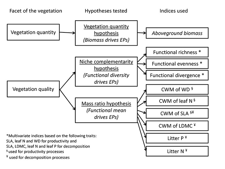
Fig. A1. Schematic representation of the two different facets of the vegetation (quality and quantity), how these translate into three testable hypotheses on alternative drivers of ecosystem process recovery and what indices are used to test each of these (see also the conceptual model in Fig. 1). EPs stands for ecosystem processes, CWM for community-weighted mean, WD for wood density, leaf N for leaf nitrogen content, SLA for specific leaf area, LDMC for leaf dry matter content, Litter P and Litter N for litter phosphorus and nitrogen content.

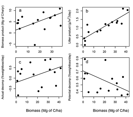
Fig. A2. Variation of each studied ecosystem process as a function of the strongest explanatory variable (highest standardized path coefficient), which was aboveground standing biomass in all four ecosystem processes (see Table A2). (a) Biomass productivity, (b) litter productivity, (c) actual litter decomposition, (d) potential litter decomposition. The fitted line is the ecosystem process as a function of the main explanatory variable, keeping the other factors contributing to the ecosystem process constant at their mean value.

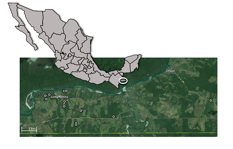
Fig. A3. Image of Mexico indicating the study location in the state of Chiapas in the white circle. Small white circles are the locations of the 15 secondary forest plots (< 1–29 yr) surrounding the village of Loma Bonita in Marques de Comillas. The continuous forest area north of the river Lacantún represents the Montes Azules Biosphere Reserve. The yellow line is the border with Guatemala. Plots of similar age (< 2 years difference) were at least 800 m apart.

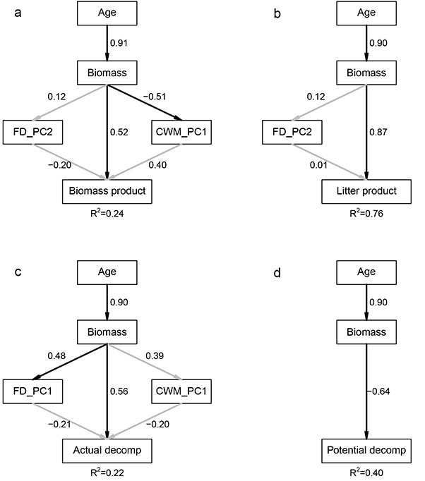
Fig. A4. Best fitting structural equation models for the four ecosystem processes when using compound variables instead of individual indicators (see Fig. 2 where individual indicators were used). As compound variables we used the principal component axes (PC1 and PC2) when secondary forest plots were separated based on their functional diversity indices (FD_PC1 and FD_PC2) and based on their community-weighted means (CWM_PC1 and CWM_PC2). See table A5 for the eigenvectors scores of the community functional properties with PC1 and PC2, note that a slightly different set of traits was used for different processes.
(a) Biomass productivity (Biomass product) was significantly explained by biomass and together with FD(PC2) and CWM(PC1) explained 24% of the variation (df = 4), (b) Litter productivity (Litter product) was explained by biomass and together with FD(PC2) explained 76% (df = 2), (c) Actual decomposition (Actual decomp) was explained by biomass and together with FD(PC1) and CWM(PC1) explained 22% of the variation (df = 4) and (d) Litter potential decomposition (Potential decomp) was explained by biomass and explained 40% (df = 1). The most suitable structural equation model presented here follows the selection criteria described in the methods, and based on different combinations of PC1 and PC2 for functional diversity and community-weighted mean indicators. Some paths are left out from the figure (unlike in Fig. 2) because this reduced the AIC based on which the best model was selected. This difference suggests that individual indicators for FD and CWM (as in Fig. 2) capture more relevant information for explaining ecosystem processes than does the use of compound variables. Black arrows represent significant relations (P < 0.05), gray arrows nonsignificant ones, given are the standardized path-coefficients.

Literature cited

Clark, D. A., S. Brown, D. W. Kicklighter, J. Q. Chambers, J. R. Thomlinson, J. Ni, and E. A. Holland. 2001. Net primary production in tropical forests: an evaluation and synthesis of existing field data. Ecological Applications 11:371–384.

Cornelissen, J. H. C. 1996. An experimental comparison of leaf decomposition rates in a wide range of temperate plant species and types. Journal of Ecology 84:573–582.

Ewel, J. J. 1976. Litter fall and leaf decomposition in a tropical forest succession in Eastern Guatemala. Journal of Ecology 64:293–308.

Janisch, J. E., and M. E. Harmon. 2002. Successional changes in live and dead wood carbon stores: implications for net ecosystem productivity. Tree Physiology 22:77–89.

Ostertag, R., E. Marín-Spiotta, W. L. Silver, and J. Schulten. 2008. Litterfall and decomposition in relation to soil carbon pools along a secondary forest chronosequence in Puerto Rico. Ecosystems 11:701–714.

Swift, M. 2004. Biodiversity and ecosystem services in agricultural landscapes? Are we asking the right questions? Agriculture, Ecosystems & Environment 104:113–134.

Wardle, D. A. 2004. Ecological linkages between aboveground and belowground biota. Science 304:1629–1633.

[Back to E096-111]