Ecological Archives E096-081-A1

Jörg G. Stephan, Johan A. Stenberg, and Christer Björkman. 2015. How far away is the next basket of eggs? Spatial memory and perceived cues shape aggregation patterns in a leaf beetle. Ecology 96:908–914. http://dx.doi.org/10.1890/14-1143.1

Appendix A. Experimental set ups, software, model description, and statistics.

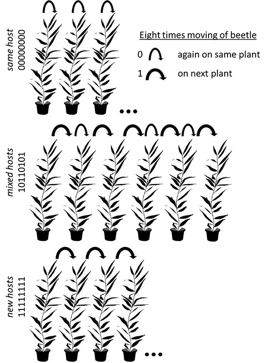
Set up of Experiment 1:

All plants in the mixed hosts and new hosts treatments could be imagined in a circle, respectively. If a beetle died/escaped the plant was excluded and the next plant in the circle was used. Therefore all mixed hosts plants were visited by 5 different females (that encountered 6 different plants) and all new hosts plants by 8 different females (that encountered 9 different plants). By distributing the change to the next plant in the mixed hosts over time we attempted to account for the fact that beetles in the later part of the experiment encountered plants with more eggs (see Appendix B: Fig. B3). In the same host treatment only plants where females laid eggs until the 9th day were used; plants where females died/escaped where excluded.

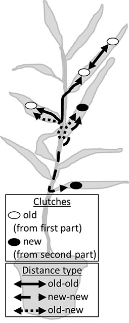
Set up of Experiment 2:

Females were allowed to lay egg clutches (old) where after the distances between these clutches were measured. Then either the same female or a female from the rearing was released again and laid clutches (new) where after the distances between these new clutches (new-new) and their relation to the already established clutches (old-new) were measured.

Picture analysis with ImageJ:

Pictures of leaves on the shoots were taken with a Canon Digital IXUS 60 while holding a white sheet of paper behind each leaf. The sheet was equipped with a piece of red tape 50 mm in length. Pictures were analyzed using ImageJ (Schneider et al. 2012). For each picture, the scale was set by using the red tape as the internal standard (draw line on 50 mm stripe → Analyze → Set Scale). Distances between clutch edge and leaf petiole were then measured on pictures of the leaf using straight lines (draw line → Analyze → Measure), and eggs within clutches were counted using the Multi-Point Tool on pictures of each clutch. For the leaf area measurements, pictures of individual leaves taken before the experiment were used. Each leaf was roughly surrounded with the Polygon Selection tool followed by removal of the outside (Edit → Clear outside). They were converted to grayscale (Image → Type → 8-bit) and made binary (Process → Binary → Make Binary) leaving the leaf in black on a white background. After measuring (and setting the Set Measurements within the Result window to Area and Limit to threshold), individual leaf areas were obtained. All commands after the selection were combined into a macro and executed with a shortcut.

Statistical analysis with R:

For the linear mixed model (LMM) and the generalized linear mixed models (GLMM), we used the function lmer and glmer from the package lme4 (Bates et al. 2012), and pair-wise comparisons were performed with the function glht from the package multcomp (Hothorn et al. 2008). Requirements for the LMM were checked visually (Zuur et al. 2009). The conditional and marginal pseudo R² values were calculated using the function r.squaredGLMM from the package MuMIn (Bartoń 2014). The analysis-of-variance tables were obtained with the function Anova from the package car (Fox and Weisberg 2011).

Model selection:

We started with full models including all interactions and used a backwards selection by removing non-significant interactions followed by non-significant main effects. The type-III analysis-of-variance tables with Wald chi-square tests were used. We included an information criterion (AIC) to show that the most parsimonious model was reached during the model selection, and the marginal R-squared (R²GLMM(m)) and conditional R-squared (R²GLMM(c)) were used to give an estimate for the absolute model fit and variance explained (Nakagawa and Schielzeth 2013) (Table A1).

Experiment 1:

The count data of the number of eggs laid on a plant and the clutch size were analyzed with a GLMM with Poisson distribution, a log link function, and each plant or each clutch nested within each plant as a Gaussian random factor for the number of eggs and the clutch sizes, respectively. Therefore, hierarchical data structures and possible model overdispersion were accounted for.

Experiment 2:

The clutch distance data were not possible to model because they were unbalanced, hierarchical (nested within each plant), not independent (each distance on each plant depended on the other distances), and were missing distance type–treatment combinations (e.g., no new-new × first release). The KS test normally also requires independent samples, but due to the lack of alternatives we decided to use this very conservative test. We did not adjust the significance levels because—contrary to many ecological studies—we had very large sample sizes that gave one mean value (Table A2). Most importantly, adjusting the significance level excludes the possibility of a Type I error but increases the likelihood of a Type II error (Moran 2003). Because the lack of overlapping standard errors indicated significant differences, we did not wanted to take the risk missing biologically relevant information. Nevertheless, correcting for multiple comparisons results in strong tendencies instead of significant comparisons (Table A3).

The proportions of leaves with and without eggs from the first female that were used by the second female on a plant were analyzed with a GLMM with a binomial distribution, a logit link function, and each observation as a Gaussian random factor. The proportion of these new clutches that were laid closer to the leaf petiole than the old clutches was analyzed with a GLMM with a binomial distribution, a logit link function, and each observation as a Gaussian random factor.

Table A1. Extended analysis-of-variance tables from generalized linear mixed models. Non-significant terms (italicized) were removed stepwise from the final model starting from the bottom row. PS = Plant Species (Salix viminalis, Salix dasyclados); T = Treatment (same host, new hosts, mixed hosts); TR = Treatment (first release, naive, experienced).

Table A2. Number of obtained distances on S. viminalis (Sv) and S. dasyclados (Sd) after the experiment. For example, ten clutches resulted in 45 interdependent distances that captured the clutch distribution of that female (distance number = (clutch number − 1) × clutch number / 2). (* only 11 of the 19 plants used received a maximum of one clutch and, therefore, there were no new–new distances).

Table A3. P values and corrected p values between pair-wise comparisons of interest for Salix viminalis (Sv) and Salix dasyclados (Sd)

Literature cited

Bartoń, K. 2014. MuMIn: Multi-model inference. R package version 1.10.0. Retrieved May 14, 2014, from http://c ran.r-project.org/package=MuMIn.

Bates, D., M. Maechler, and B. Bolker. 2012. lme4: Linear mixed-effects models using S4 classes.

Fox, J., and S. Weisberg. 2011. An {R} Companion to Applied Regression. Sage Publications.

Hothorn, T., F. Bretz, and P. Westfall. 2008. Simultaneous inference in general parametric models. Biometrical Journal 50:346–363.

Moran, M. 2003. Arguments for rejecting the sequential Bonferroni in ecological studies. Oikos 2:403–405.

Nakagawa, S., and H. Schielzeth. 2013. A general and simple method for obtaining R 2 from generalized linear mixed-effects models. Methods in Ecology and Evolution 4:133–142.

Schneider, C., W. Rasband, and K. W. Eliceiri. 2012. NIH image to imageJ: 25 years of image analysis. Nature methods 9:671–675.

Zuur, A. F., E. N. Ieno, N. J. Walker, A. A. Saveliev, and G. M. Smith. 2009. Mixed effects models and extensions in ecology with R. Genetics. Springer Verlag.

[Back to E096-081]