Ecological Archives E096-073-A3

Helen C. Wheeler, Toke T. Høye, Niels Martin Schmidt, Jens-Christian Svenning, and Mads C. Forchhammer. 2015. Phenological mismatch with abiotic conditions—implications for flowering in Arctic plants. Ecology 96:775–787. http://dx.doi.org/10.1890/14-0338.1

Appendix C. Random effects analysis of contributions of timing of flowering to temperatures experienced during development and associations between timing of flowering and flower abundance.

Here we summarize the associations between plot, year and timing of flowering (Table C1). There is a strong association between timing of flowering and plot and year. In Dryas and Salix more variation in timing of flowering is driven by plot differences, whereas in Cassiope and Papaver more variation in timing of flowering is driven by interannual variation. Correlation between predictor variables and random effects creates bias in random effects models and therefore in our main analysis we include only these fixed effects. However for completeness we also show these random effects models, which are analogous to the fixed effects models in the main manuscript but include random effects of year and plot.

We suggest that these random effects models are highly conservative due to shrinkage of estimates towards the mean, which, given the strong association between timing of flowering and plot and year, diminishes our ability to discern the effects of timing of flowering. This is demonstrated in Table C2 and C3, where we observe a reduction in ∆AICc and also observed in an increase in the residual variance of many of our models when we add our timing of flowering fixed effect to the model, which is characteristic of issues with correlated predictors and random effects (Gelman and Hill 2007). We provide an example of these biases for by plotting our random effects models for our first analysis (Fig. C1).

Despite this, the best models (associated with the lowest AICc) remain the same as in our main fixed effect analysis in most cases, reflecting the strong nature of these trends. For Cassiope, Dryas, and Papaver we find a contribution of timing of flowering to freezing exposure prior to flowering, for Salix, models are sufficiently similar we are unable to discern between models with and without a contribution of timing of flowering. For Dryas and Salix we find a contribution of timing of flowering to temperature during flowering. For Papaver we are unable to discern between models with and without a contribution of timing of flowering, and for Cassiope only summer temperature was associated with mean temperature during flowering (Table C2).

In our mixed model analysis of the association between timing of flowering and flower abundance in all cases the selected models are the nulls (Table C3). This reflects the relatively weak relationship between timing of flowering and flower abundance. The relationship we found between timing of flowering and flower abundance is lost when random effects of plot and year are added as addition of these random effects which are highly correlated with our predictor weaken the observed relationship such that is can no longer be observed. We argue that this consequence of addition of these random effects and their correlation with our main effects rather than the absence of an ecological relationship between timing of flowering and flower abundance.

Table C1. Summary of associations between timing of flowering and plot and year. Adjusted R² values from one way ANOVAs (first two columns) and a two-way ANOVA modeling both plot and year effects (final column) are shown.

Table C2. Summary of generalized additive models of exposure to freezing temperature (left) and mean temperature during flowering (right) with random effects of plot and year included. Models with the lowest AICc values for each model set are indicated in bold. Where models differ by less than ∆AICc=1 there are considered equally well supported and all such models are indicated in bold. The percentage of deviance explained by each model is shown. Estimates for the effects of spring and summer temperatures (± 1 SE) are also shown for each model.

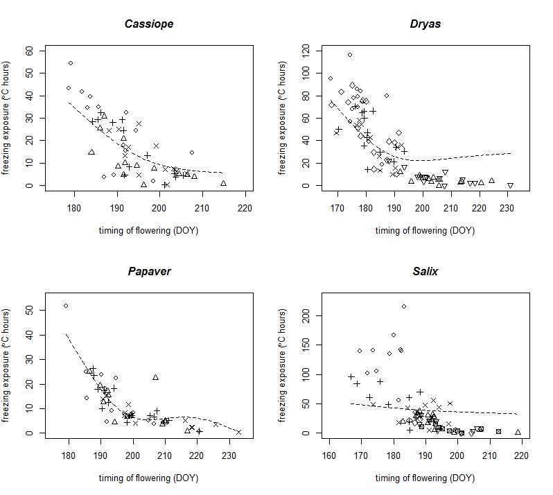
Fig. C1. Relationship between the date of peak flowering and exposure to freezing conditions (degree hours below 0°C prior to flowering onset) in four flowering species from Zackenberg. We plot analogous models to those presented in Fig. 2, for comparison. Symbols denote different plots. The line shows the smoothed relationship fitted using a generalized additive model with random effects of plot and year. Biases in GAM splines relative to models without random effects can be observed by comparing these to Fig. 2.

 Table C3. Summary and comparison of models of the association between the timing of flowering and flower abundance; effect sizes are given in addition to whether a plot effect is included in the model. Best models are indicated by an asterisk (*).

Literature cited

Gelman, A., and J. Hill. 2007. Data analysis using regression and multilevel/hierarchical models. Cambridge, UK, p480–481.

[Back to E096-073]