Ecological Archives E096-072-A5

Petr Pyšek, Ameur M. Manceur, Christina Alba, Kirsty F. McGregor, Jan Pergl, Kateřina Štajerová, Milan Chytrý, Jiří Danihelka, John Kartesz, Jitka Klimešová, Magdalena Lučanová,10 Lenka Moravcová, Misako Nishino, Jiří Sádlo, Jan Suda, Lubomír Tichý, and Ingolf Kühn. 2015. Naturalization of central European plants in North America: species traits, habitats, propagule pressure, residence time. Ecology 96:762–774. http://dx.doi.org/10.1890/14-1005.1

Appendix E. Missing data imputation procedure and results.

Several variables in our data set had between 0.2 and 36% of entries missing (Table E1). To handle missing data we used multiple imputation rather than case-wise deletion of incomplete entries. We did this because case-wise deletion results in information loss (in our case reducing the taxa available for analysis from 466 to just 176), reduced statistical power and potentially biased parameter estimates (Rubin 1976). These problems become more important if data are missing for some underlying reason linked to the biology or geography of the species (Nakagawa and Freckleton 2011).

Table E1. List of variables used in imputation and the fraction of entries missing for each variable and the transformation applied in Amelia before imputation.

Note: n.a. means not applicable, as no transformation was performed.

We performed multiple imputation and model diagnostics in R 2.15.2 (R Core Team, 2012) using the Amelia II package (Honaker et al. 2011). Multiple imputation involves imputing m values for each missing cell in the data set, creating m complete data sets where the observed values are the same but the missing values are filled using a distribution of values that reflect the uncertainty around those missing values. Amelia II performs multiple imputation using an EMB algorithm (Expectation-Maximization-algorithm and Bayesian classification model). This method of imputation has advantages over ad-hoc methods such as mean imputation, which can lead to serious biases in variances and covariances (Honaker et al., 2011). In order to meet the assumption of multivariate normality required for Amelia II we transformed continuous numeric variables using either the natural logarithm or the square root transformation (Table A1). To better meet the assumption that variables are missing at random we aimed to use the full data set for imputation, including response variables. However, we had to exclude latitudinal range and longitudinal range because these variables were highly correlated with each other and with several others, causing Amelia's EMB algorithm to fail.

We imputed five data sets (following Honaker et al., 2011). Because we found that each of the five imputed data sets had a very different number of iterations (number of iterations ranged from 54–136) we re-ran the imputation, this time setting the ridge prior to 1% of the number of observations in the data set (n = 446) as recommended by Honaker et al. (2011). This did not improve the evenness in the number of iterations (number of iterations ranged from 36–166) or the diagnostic plots. Therefore, we decided to use the imputed data sets that had been calculated without a ridge prior in further analyses.

Diagnostic plots for imputed data sets

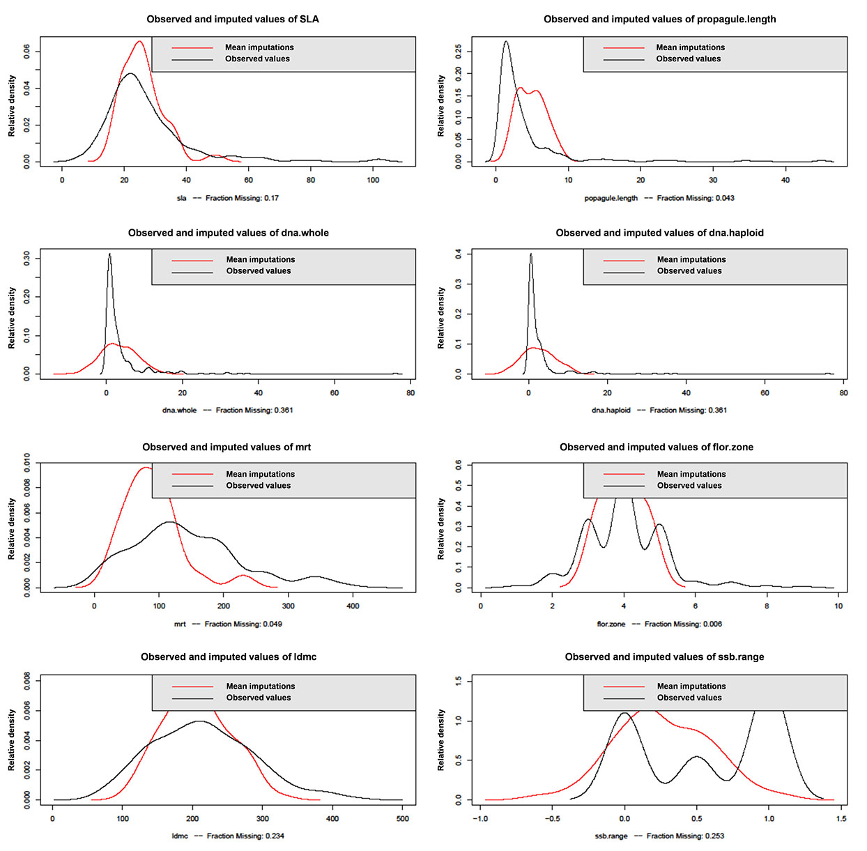
Amelia provides plots to check the plausibility of the imputation model by comparing the distribution of imputed and real values. For each cell that is missing in a variable the diagnostic will find the mean of that cell across each of the m data sets and use that value for the density plot. However, there may be no reason to expect a priori that the distributions will be identical, so these plots are not a definitive test. We can however check to see whether the imputed distributions are a reasonable shape and that they peak within the known bounds of the actual distribution of the data (Abayomi et al. 2008).

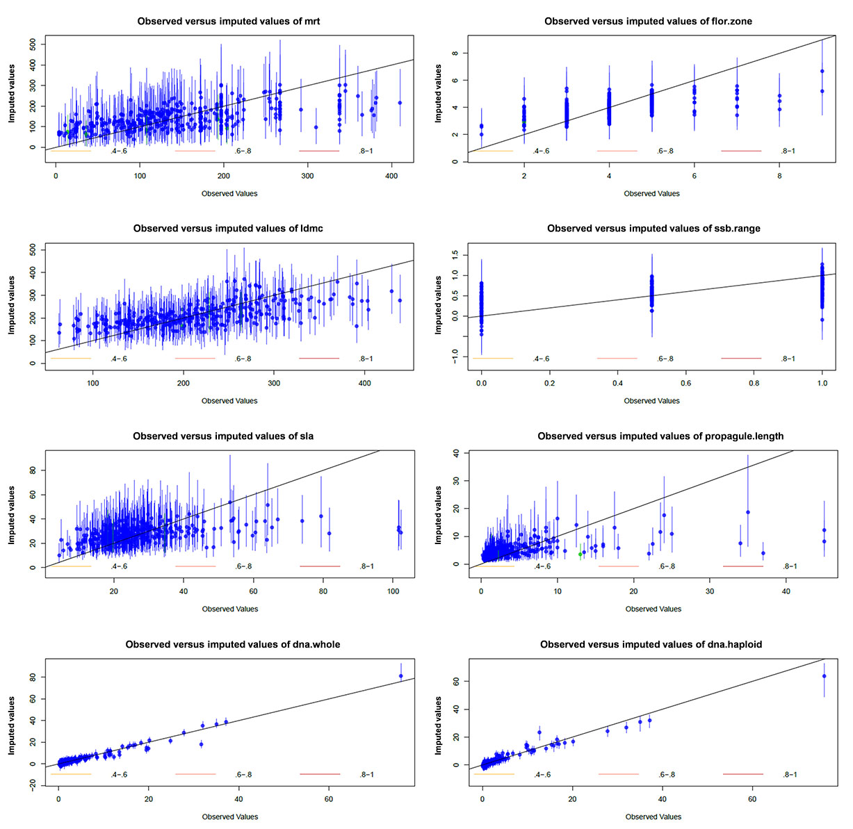
First, the imputation model appears to predict new values that are within the known limits of our data (Fig. E1). Second, the other diagnostic test available in Amelia II is a function called overimpute. This assesses how accurate the imputed data is by sequentially treating the observed values as if they were missing and generating several hundred imputed values (allowing the construction of confidence intervals) for them as if they were in fact missing. The results of this simulation can be examined graphically. If the true and observed values' confidence intervals cross the x = y line (imputation perfectly agrees with actual data) then the imputation model is doing well. Fig. E2 shows that for variables with high missingness (dna.whole and dna.haploid) the imputation model predicts values that generally agree with the actual data available in that variable, but the confidence intervals are small and do not always cross the x = y line. For minimum residence time (mrt), leaf dry matter contend (ldmc), specific leaf area (sla) and propagule length (propagule.length) it is clear that at the upper end of the distribution of those variables the predicted values from the imputation model do not agree with actual values. However, for the majority of the distribution of those variables the imputation model agrees with the observed data relatively well.

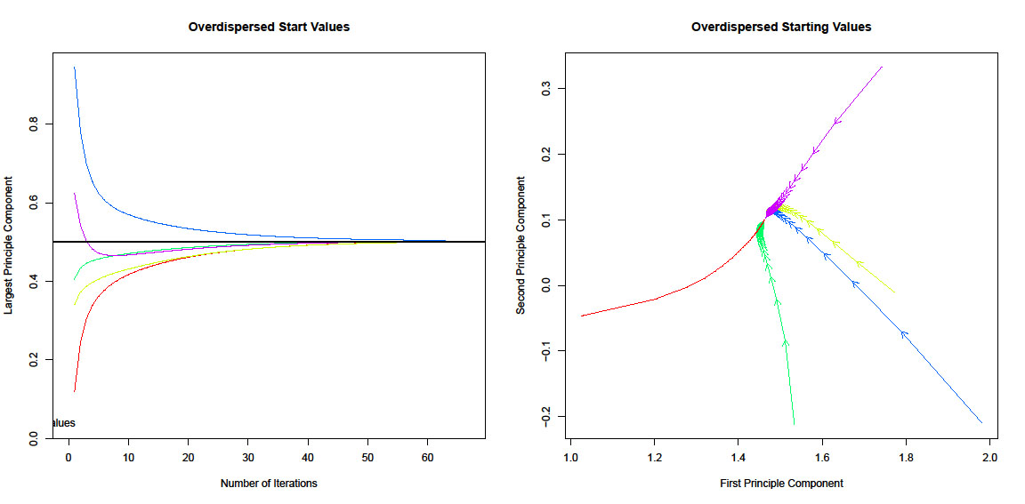
We used the disperse function to test whether the analysis converged on the global maximum of the likelihood surface and starting values. This diagnostic runs EM chains from multiple starting values that are overdispersed from the estimated maximum. We found that the EM algorithm had converged on the global maximum of the likelihood, indicating that Amelia was in the right parameter space when choosing starting values for imputation runs (Fig. E3).

Fig. E1. Comparative plots of densities between observed values for continuous numeric variables and the mean of the imputed values across each of the m data sets (m = 5). Categorical variables, variables without missing cases and variables with < 2 missing cases are not plotted.

Fig. E2. Overimputation diagnostic plots showing mean and 90% confidence intervals indicate where imputed values would lie if they were missing in the data set.

Fig. E3. Overdispersion diagnostic plot indicating that all the chains from the expectation-maximization algorithm have converged to the same parameter estimates (i.e., achieved a global maximum not a local one for the likelihood function).

Literature cited

Abayomi, K., A. Gelman, and M. Levy. 2008. Diagnostics for multivariate imputations. Journal of the Royal Statistical Society, Series C – Applied Statistics, 57:273–291.

Honaker, J., G. King, and M. Blackwell. 2011. Amelia II: A program for missing data. Journal of Statistical Software 45. URL: http://www.jstatsoft.org/v45/i07/paper.

Nakagawa, S., and R. P. Freckleton. 2011. Model averaging, missing data and multiple imputation: a case study for behavioural ecology. Behavioral Ecology and Sociobiology 65:103–116.

R Core Team. 2012. R: A language and environment for statistical computing. R Foundation for StatisticalComputing, Vienna, Austria. URL http://www.R-project.org/.

Rubin, D. B. 1976. Inference and missing data. Biometrika 63:581–592.

[Back to E096-072]