Ecological Archives E096-060-A1
Jill R. Welter, Jonathan P. Benstead, Wyatt F. Cross, James M. Hood, Alexander D. Huryn, Philip W. Johnson, and Tanner J. Williamson. 2015. Does N2 fixation amplify the temperature dependence of ecosystem metabolism? Ecology 96:603610. http://dx.doi.org/10.1890/14-1667.1
Appendix A. Detailed temperature manipulation and experimental channel methods description and statistical output from mixed-effects model selection.
A.1 Temperature manipulation and experimental channels
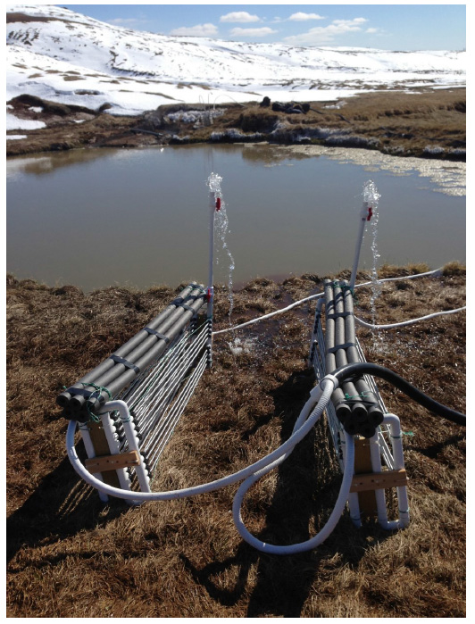
Our experimental temperature gradient was achieved using a gravity-fed, geothermal heat-exchange system that supplied an array of streamside channels. The heat exchangers were fed cool water (mean temperature 7.5°C, ~1 L/s) via a 50.8-mm flexible polyvinyl chloride (PVC) pipe placed in an unnamed tributary of the Hengladalsá River. This cool water supply was diverted into three 25.4-mm flexible PVC pipes. Cool water in one of these pipes was routed to a heat exchanger (see Fig. A1) deployed in a spring-fed geothermal pool (mean temperature 30.1°C) that warmed the water to ~10°C above ambient. The second cool water supply was routed through an identical heat exchanger in the same pool. Warm water leaving the second exchanger supplied a third heat exchanger in an adjacent hot spring (mean temperature 62.5°C; see Fig. A2). This heat exchanger warmed water to ~20°C above ambient. The third cool water supply was unheated.
We mixed water from the three water supplies to achieve five treatments ranging in mean daily temperature from 7.5°C to 23.6°C (mean ± 1 SD: 7.5 ± 1.8°C, 11.2 ± 1.8°C, 15.5 ± 1.9°C, 19.0 ± 1.8°C, 23.6 ± 2.0°C; Appendix, Table A1). Treatments were delivered to five constant-head tanks (modified 45-L coolers), which supplied 15 experimental channels (n = 3 at each temperature, molded PVC, length 3 m, width 25.4 mm, wall height 40 mm). Channels were un-shaded, faced due south, and divided into three blocks with the five temperatures randomized within each block (Fig A3). Each channel contained a temperature data logger (HOBO Pendant UA-002-08; Onset Computer Corp., Bourne, MA, USA) at its upstream end. Mean flow rate was 0.03 L/s (mean depth 6 mm, mean water velocity 0.24 m/s).
Table A1. Summary statistics describing the temperature regime and source water chemistry in the 5 treatments: mean increase in temperature (°C) relative to the ambient treatment, mean daily temperature (°C, ± 1 SD), mean daily temperature range (°C), ammonium (μg/L, ± 1 SD), nitrate (μg/L, ± 1 SD) and soluble reactive phosphorus (SRP) (μg/L, ± 1 SD).
Treatment |
Increase over |
Daily mean |
Mean daily |
NH4+ |
NO3-N |
SRP |
A |
- |
7.5 (1.8) |
4.4 |
11.6 (7.1) |
52.2 (44.2) |
16.6 (7.8) |
B |
3.8 |
11.2 (1.8) |
3.8 |
7.0 (4.7) |
37.0 (31.3) |
19.0 (6.8) |
C |
8.1 |
15.5 (1.9) |
3.6 |
11.5 (5.5) |
46.0 (40.6) |
15.3 (4.0) |
D |
11.4 |
19 (1.8) |
3.9 |
7.5 (5.1) |
45.2 (44.3) |
18.6 (8.7) |
E |
16 |
23.6 (2.0) |
3.8 |
11.8 (7.3) |
41.2 (43.2) |
15.4 (7.3) |
Table A2. Mixed-effects modeling of the effects of temperature and biomass on areal rates of GPP and ER; N[total] = 26, N[channel] = 15 SE, standard error; SD, standard deviation; AICc, Akaike Information Criterion for small samples; R²GLMM(m), marginal R² for fixed factors; R²GLMM(c), conditional R² for both fixed and random factors. Models were fit with the R function 'lme' from the package 'nlme' (Pinheiro et al. 2014). AICc values were calculated using ML, while other parameters were from REML estimations. R²GLMM(m) and R²GLMM(c) were estimated with the R function 'r.squaredGLMM' from the package 'MuMIn' (Bartoń 2014), following Nakagawa and Schielzeth (2013). * P < 0.05, ** P < 0.01, *** P < 0.001.
|
loge GPP models |
loge ER models |
||||
Model name |
Null |
Temperature |
Biomass |
Null |
Temperature |
Biomass |
Fixed effects |
b (SE) |
b (SE) |
b (SE) |
b (SE) |
b (SE) |
b (SE) |
|
4.40 (0.36)*** |
87.31 (5.07)*** |
-7.08 (0.88)*** |
3.05 (0.31)*** |
71.28 (3.21)*** |
-5.95 (0.82)*** |
|
– |
-2.13 (0.13) *** |
– |
– |
-1.73 (0.08)*** |
– |
|
– |
– |
1.11 (0.09)*** |
– |
– |
0.99 (0.08)*** |
|
– |
0.06 (0.01) *** |
0.03 (0.01)*** |
– |
0.02 (0.01) |
0.00 (0.01) |
Random effects |
SD |
SD |
SD |
SD |
SD |
SD |
|
0.86 |
1.53 |
1.31 |
0.75 |
2.50 |
1.02 |
|
0.03 |
0.03 |
0.02 |
0.02 |
0.05 |
0.02 |
|
0.55 |
0.27 |
0.21 |
0.50 |
0.19 |
0.35 |
R²GLMM(m) |
– |
0.91 |
0.87 |
– |
0.86 |
0.87 |
R²GLMM(c) |
0.86 |
0.96 |
0.98 |
0.86 |
0.98 |
0.92 |
AICc |
88.60 |
38.93 |
41.83 |
86.29 |
38.66 |
47.05 |
Fig. A1. Two large heat exchangers prior to deployment in the warm spring in the background. Photo credit: Jonathan P. Benstead.
Fig. A2. Spiral heat exchanger being lowered into the 62.5°C hot spring. Photo credit: Jonathan P. Benstead.
Fig. A3. Experimental channels with header tanks in the background. Photo credit: Jonathan P. Benstead.
Fig. A4. Chambers used to measure gross primary production, community respiration, and nitrogen fixation on experimental tiles. Photo credit: Jonathan P. Benstead.
Fig. A5. Mean stream water temperature in the five treatments for a one-week period (11–17 July 2014).
Literature Cited
Bartoń, K. 2014. MuMIn: Multi-model inference. R package version 1.10.0.
Nakagawa, S., and H. Schielzeth, 2013. A general and simple method for obtaining R² from the generalized linear mixed-effects models. Methods in Ecology and Evolution 4:133–142.
Pinheiro J., D. Bates, S. DebRoy, D. Sarkar, and R Core Team. 2014. nlme: Linear and Nonlinear Mixed Effects Models_. R package version 3.1-117.