Ecological Archives E096-031-A1

Jennifer C. McGarvey, Jonathan R. Thompson, Howard E. Epstein, and Herman H. Shugart, Jr.. 2015. Carbon storage in old-growth forests of the Mid-Atlantic: toward better understanding the eastern forest carbon sink. Ecology 96:311–317. http://dx.doi.org/10.1890/14-1154.1

Appendix A. Detailed methods of study area and site selection, field methods, data processing and analysis, and the comparison of old growth sites to the surround forest matrix.

Study area and site selection

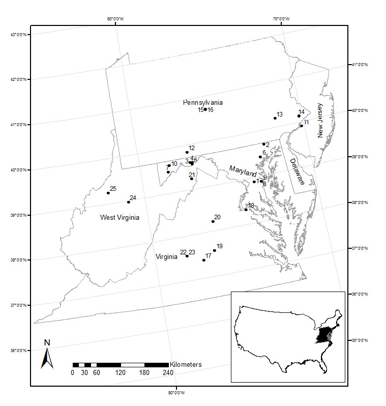
We defined the Mid-Atlantic as Virginia, Delaware, and Maryland, and parts of West Virginia, Pennsylvania, and New Jersey (Fig. A1). The climate is humid and warm, with growing seasons ranging from 100 to 250 days (Stolte et al. 2012). Forest is the prevailing land cover type in the region, dominated by oak/hickory (Quercus spp. and Carya spp.), maple/beech/birch (Acer spp., Fagus grandifolia Ehrh., and Betula spp.), and oak/pine (Pinus spp.) forest community groups (McKenney-Easterling et al. 2000). Quercus alba L. (white oak), Q. velutina Lam. (black oak), Q. prinus L. (chestnut oak), Q. rubra L. (northern red oak), Castanea dentata (Marsh.) Borkh. (American chestnut), Pinus spp., Ulmus spp. and Carya spp. dominated pre-settlement forests (Whitney 1996, Abrams 2003), and with the exception of Castanea dentata these species still are common in the old growth forests of the region (Thompson et al. 2013).

There are multiple definitions of old growth for eastern temperate forests based on stand structure and successional processes (e.g., Foster et al. 1996, Wirth et al. 2009, Hoover et al. 2012). No clear ecological thresholds regarding disturbance frequency or age exist across these definitions, and so identification of old growth can be problematic. To simplify initial site selection, and to account for variability in disturbance history across sites, we broadly define old growth as forests believed to have a stand age of ≥ 150 years (Cogbill 1996). Our goal was to measure all old growth sites known to exist in the Mid-Atlantic that are not anomalous due to their edaphic or topographic setting. We reviewed all academic and gray literature on old growth remnants in the region with reported stand ages. The majority of these stands were described in Davis (1996) and Kershner and Leverett (2004); others were identified sites in conversation with state forest agencies, and conservation and land trust associations (e.g., The Nature Conservancy). A total of 35 sites were identified for field visits. Ten of these sites were deemed unusable either due to recent natural or anthropogenic disturbance (e.g., gypsy moth outbreaks, timber harvesting) which caused large-scale mortality in the dominant overstory trees, or because the site was inaccessible or not representative of the greater Mid-Atlantic region. Twenty-five sites were sampled during summer 2012 (Fig. A1).

Field methods

Stand boundaries were delineated following the methods of Wirth et al. (2009), which utilizes: (1) the abundance of large, old stems, (2) abundance of standing and fallen dead wood at various stages of decay, (3) relatively few signs of anthropogenic disturbance, (4) a multi-layered canopy, and (5) canopy gaps. Emphasis was placed on the first three characteristics, because they are easily recognized within an older stand, and contrast strongly with conditions of younger forests. Additionally, the stand needed to be of sufficient area to fit three 0.07 ha sampling plots. In practice, defining the stand edge was difficult. We were conservative in our classification and erred towards identifying forest as secondary over old growth.

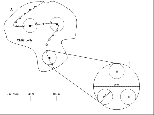
We established sampling points at 15-m intervals along a transect oriented to cover the greatest possible area of each stand (Fig. A2). Subsequently, transect length varied among sites. We estimated total basal area (BA; m²/ha) of all stems within a variable radius of all sampling points using a 10-factor prism. This BA estimation technique was intended to capture the range of structural variability present within the stand. We then took detailed plot measurements within 15-m radius circular plots centered at three to four sampling points that represented the 10th, 50th, and 90th quantiles in terms of prism-estimated BA. For sites with four sampling points, two points represented the 50th quantile. Although we used prism-estimated BA to select plots, we did not stratify plots by BA prism estimates in subsequent analysis because BA prism estimates proved ineffective at estimating measured plot-level BA. Instead, analysis was based on site averages. At the center of each plot, we recorded aspect, slope, and geographic coordinates.

Within each plot, we recorded the species, height, and DBH (diameter-at-breast-height; 1.37 m) of all live woody stems ≥ 5 cm DBH, and species and DBH for all stems 1-5 cm DBH within three non-overlapping 5-m radius subplots nested within the larger plot. We measured dead wood volume using field protocols developed by Harmon and Sexton (1996). We classified all dead wood as a log, snag, or stump. For logs (≤ 45° relative to the ground), we measured the diameters at both ends and the midpoint, and the length of the piece of wood; for snags (> 45° relative to the ground and > 1.37 m height), the DBH and height; for stumps (> 45° relative to the ground and < 1.37 m height), the length, and top and base diameters. We identified decay classes using the categories described by Waddell (2002). Following McGee et al. (1999), all large dead wood (≥ 25 cm diameter) in the 15 m radius plots and medium dead wood (10–25 cm diameter) in the subplots were inventoried.

To estimate maximum age of the plots, one tree core each was collected from two to three of the dominant canopy stems from each plot for a total of ten cores per site, taken at 1.37-m along the mid-slope of the tree. At four sites, heart rot in canopy stems prevented the collection of complete cores for the largest trees. Large stems (> 50 cm DBH) with rot ranged from 6 to 29% of all stems in their size class at the four sites. Cores were collected from the next largest stems without rot. We used a 40.6 cm borer and were unable to reach the center of some of the larger trees, and did not attempt to estimate missing rings. Due to ecological or historical significance, landowners denied permission to collect cores at nine sites. However, reliable stand age data were available for all but one of these sites (Table A1). We dried, mounted, and sanded all samples, then estimated maximum plot age by counting tree-rings under a Wild M8 stereozoom microscope, and cross-dated counts by comparing shared narrow rings across cores (Yamaguchi 1991). We selected the oldest tree at each site as an estimate of maximum site age, hereafter referred to as "oldest tree age."

At the center of two randomly chosen subplots within each plot, we collected leaf litter and soil from the O horizon within a 0.1-m² frame at 23 of the 25 sites. The frame method (Burton and Pregitzer 2008) worked best for the generally rocky soils or shallow O horizons at the majority of field sites. We took five soil cores using a 2.5 cm diameter corer to determine the mean depth of the O horizon at each sampling point. For a subsample of all sites (n = 5), we collected a separate 0.01 m² sample at each sampling point to estimate bulk density. Bulk densities of the O horizon were not significantly different across the five sites (one-way ANOVA; df = 4, f = 2.316, p = 0.095), and so a mean of 0.19 g/cm³ was assumed for all sites. In the lab, we passed the samples through a 2-mm sieve to remove roots and other large organic matter, dried them at 105°C for 24 hours, and finely ground them using a ball mill. We obtained estimates for percentage of carbon (C) from each sample using a CE elemental analyzer (CE Elantech, Inc., Lakewood, NJ).

Data processing

Estimates of live aboveground C (AGC) were based on generalized allometric equations developed by Jenkins et al. (2003) and Lambert et al. (2005). These equations were developed for broad-scale use, however are underdeveloped for large and old trees. Equations developed by Jenkins et al. (2003) are based on hardwood stems with maximum DBH of 56 to 73 cm and do not address how the distribution of biomass changes throughout the life cycle of a stem (Peichl and Arain 2007). As identified by Ahmed et al. (2013), Lambert et al. (2005) use a more statistically rigorous approach than Jenkins et al. (2003); However, the Lambert et al. (2005) allometries lack specific equations for some important Mid-Atlantic species, most notably Liriodendron tulipifera. In general, the Lambert et al. (2005) equations produced slightly lower biomass estimates than Jenkins et al. (2003). As neither set of regressions stood out as superior, we used the mean biomass estimate of the two methods. For all woody biomass, we assumed C to be 50% of biomass (Alexeyev and Birdsey 1998) or Nelson et al. 2000.

We used different equations for volumetric estimates of dead wood based on the dead wood classification and measurements for each dead wood type (Harmon and Sexton 1996). For logs, we used the Newton formula which requires three diameter measurements:

Where L is length, A_b, A_m, and A_t are area at the bottom, middle, and top, respectively. For stumps, we used the formula for a frustrum of a cone:

For snags, we used a modified Huber formula (Wenger 1984) for a cylinder:

Of the three volume equations, the Huber formula is the most simplified and potentially more prone to error in estimating true volume. Dead wood pieces are generally irregular in shape, and error in volume estimates increase with fewer diameter measurements collected. However, this formula has been shown to provide unbiased estimates (Van Wagner 1968, Brown 1971), and so we used the Huber formula to approximate true snag volume. To estimate dead wood biomass, we used the equation from Waddell (2002):

Where V is volume, SpG is the specific gravity of fresh wood that varies by species, and DCR is the decay class reduction factor, which reduces the specific gravity of wood by decay class. The following four decay class reduction factors were used: II = 0.78 (softwood = 0.84) g/cm³, III = 0.45 (0.71), and IV & V = 0.42 (0.45) g/cm³ developed by Waddell (2002) from an assessment of dead wood biomass in FIA plots.

We calculated the mass of C in the O horizon using Amundson (2001):

Where M_O is the C mass, C_O is the C concentration, BD_O is bulk density, and z_O is the depth of the O horizon.

Data analysis

We used linear regression to model relationships between maximum tree age and C stocks. Where linear trends explained significant variability around the mean or when the C pool stored at least 10% of stand level C, we further explored more defined aspects of structure to determine possible causes for the presence (or absence) of a significant relationship. If the oldest tree age/C relationship was insignificant, but the pool contained at least 10% of stand level C, other environmental variables were included in a multivariate model of biomass to improve the relationship. Environmental variables used included slope, aspect, elevation, and topographic wetness index (TWI). TWI values of seven or less indicates the most xeric conditions and ten indicates the most mesic conditions (Moore et al. 1993). To select a parsimonious linear model of C, we used stepwise model selection with backward elimination (McCune and Grace 2002). After predictor elimination, the current and previous models were compared using analysis-of-variance tables to test whether the model terms were significant. We also used linear regression to explore relationships among different C pools, when the C pool(s) stored at least 10% of stand level C.

We explored relationships between AGC and structural variables across live stem diameters and maximum dead wood diameters. To identify the importance of species composition in driving structural characteristics in old growth, we objectively described the similarity among forests in terms of tree composition by a two-way hierarchical agglomerative cluster analysis with Ward's agglomeration (McCune and Grace 2002) using the vegdist function in the vegan package (Oksanen et al. 2011) of the R statistical software (R Development Core Team 2014). We summarized species composition and abundance using relative BA (RBA = individual species BA / Σ BA of all species). Sites were grouped based on compositional dissimilarity and measured using Sørensen distance. By examining the resulting dendrogram and the percentage of information remaining after the formation of each cluster we settled on four groups. We then use a variety of descriptive statistics to compare variation in live and dead AGC across stem size classes for all sites and by species composition.

Comparison of old growth sites to the surrounding forest matrix

To understand how the mature and old growth stands compare to the matrix of younger forests in the Mid-Atlantic, we plotted live and dead AGC against regional averages obtained from the U.S. Forest Service Forest Inventory and Analysis (FIA) program, which monitors a national network of forest plots (for details on the FIA field protocol see http://www.fia.fs.fed.us). We queried all forested FIA plots from the Mid-Atlantic study region for values of live and dead AGC for plots inventoried in 2011 (n = 1855). Live AGC was calculated using Jenkins et al. (2003) allometric equations and dead AGC included only wood. AGC was broken down by oldest tree age, and bins were ten years. We plotted the mean values and standard deviations of the FIA plots with the old growth sites to qualitatively describe the relationship between AGC and oldest tree age across secondary succession. In this way we employed an informal chronosequence approach with a space-for-time substitution to infer changes in C storage through secondary succession. Differences in plot design, study area, and sampling methods between this study and the FIA data preclude any formal statistical analysis, and so the informal chronosequence is solely a qualitative way of contextualizing the old growth sites.

Table A1. Summary table of C stores for all twenty-five old growth sites. Also included are oldest tree age, forest type delineated by a agglomerative clustering algorithm, and relative C stored in the four pools.

(A) J. Parker, personal communication; (B) Ruffner and Abrams 1998; (C) Rucker 2001; (D) Nowacki and Abrams 1994; (E) Druckenbrod et al. 2005; (F) Dierauf 2011; (G) Rentch et al. 2003.

Table A2. Definitions of USDA-NRCS species codes.

Fig. A1. Location of the twenty-five old growth forests sampled within the Mid-Atlantic study area. See Table A1 for key to site codes.

Fig. A2. An example of transect and plot layout for old growth field sampling. (A) Within each stand, a transect (dashed line) was oriented to cover the maximum possible area within the stand boundary (solid line). BA was estimated at sampling points (empty squares) placed 15-m apart along the transect. From these BA estimates, three to four 30-m diameter plots (circles) were placed at sampling points. The number of plots depended on size of the stand. (B) Within each plot, all large dead wood and live stems greater than 5 cm DBH were recorded, and slope and aspect were measured at the center of the plot. Additionally within each plot, three 10-m diameter subplots (small circles) were surveyed for medium dead wood and live stems 1–4.9 cm DBH. Soil O horizon and leaf litter samples were collected from 0.9 m² quadrats (squares) at the center of two randomly selected subplots.

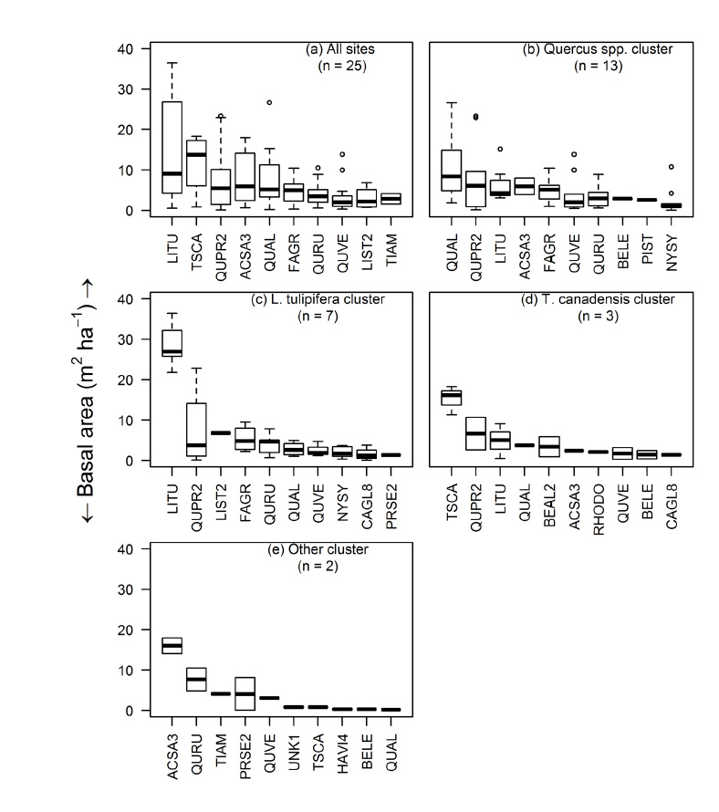
Fig. A3. Box plots of basal area (m²/ha) of the ten most dominant species across sites. Sites are characterized by their cluster groups delineated by a agglomerative clustering algorithm. Cluster names are based on the most dominant species by basal area. See Table A2 for species codes.

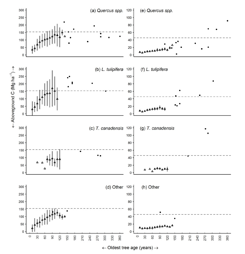
Fig. A4. Relationship between oldest tree age and (a–d) live AGC; and (e–h) dead AGC for U.S. Forest Service inventory plots in ten year age class bins (triangles) and twenty-five old growth stands (dots). Forest types reflect the tree species composition of each old growth stand identified by a cluster analysis. Each plot represents stands that fall into an associated forest type. FIA forest types that best approximated the old growth species composition were used: Yellow-poplar/white oak/northern red oak for the Quercus spp. group, Yellow-poplar for the Liriodendron tulipifera group, Eastern hemlock for the Tsuga canadensis group, and Sugar maple/beech/yellow birch for the Other group. Bars represent one standard deviation. The grey dashed lines indicate the mean live and dead AGC values, respectively, across old growth sites.

Literature cited

Abrams, M. D. 2003. Where Has All the White Oak Gone? BioScience 53:927–939.

Ahmed, R., P. Siqueira, S. Hensley, and K. Bergen. 2013. Uncertainty of Forest Biomass Estimates in North Temperate Forests Due to Allometry: Implications for Remote Sensing. Remote Sensing 5:3007–3036.

Alexeyev, V., and R. A. Birdsey. 1998. Carbon storage in forests and peatlands of Russia.

Amundson, R. 2001. The carbon budget in soils. Annual Review of Earth and Planetary Sciences 29:535–562.

Brown, J. 1971. A planar intersect method for sampling fuel volume and surface area. Forest Science 17:96–102.

Burton, A. J., and K. S. Pregitzer. 2008. Measuring Forest Floor, Mineral Soil, and Root Carbon Stocks. Pages 129–142 in C. M. Hoover, editor. Field Measurements for Forest Carbon Monitoring. Springer Science, New York, New York, USA.

Cogbill, C. V. 1996. Black growth and fiddlebutts: the nature of old growth red spruce. Eastern old growth forests. Island Press, Washington, DC, USA:113–125.

Davis, M. B. 1996. Old Growth in the East: A Survey. Island Press, Washington D.C., USA.

Dierauf, T. A. 2011. History of the Montpelier Landmark Forest: Human disturbance and forest recovery.

Druckenbrod, D. L., H. H. Shugart, and I. Davies. 2005. Spatial Pattern and Process in Forest Stands within the Virginia Piedmont. Journal of Vegetation Science 16:37–48.

Foster, D. R., D. A. Orwig, and J. S. McLachlan. 1996. Ecological and conservation insights from reconstructive studies of temperate old growth forests. Tree 11:419–424.

Harmon, M. E., and J. Sexton. 1996. Guidelines for measurements of woody detritus in forest ecosystems. LTER Network Office, University of Washington, Seattle, Washington, USA.

Hoover, C. M., W. B. Leak, and B. G. Keel. 2012. Benchmark carbon stocks from old growth forests in northern New England, USA. Forest Ecology and Management 266:108–114.

Jenkins, J. C., D. C. Chojnacky, L. S. Heath, and R. A. Birdsey. 2003. National-scale biomass estimators for United States tree species. Forest Science 49:12–35.

Kershner, B., and R. T. Leverett. 2004. The Sierra Club Guide to the Ancient Forests of the Northeast. First edition. Sierra Club Books, San Francisco, Claifornia, USA.

Lambert, M., C. Ung, and F. Raulier. 2005. Canadian national tree aboveground biomass equations. Canadian Journal of Forest Research 35:1996–2018.

McCune, B., and J. Grace. 2002. Analysis of ecological communities (Gleneden Beach, OR: MjM Software Design).

McGee, G. G., D. J. Leopold, and R. D. Nyland. 1999. Structural Characteristics of Old growth, Maturing, and Partially Cut Northern Hardwood Forests. Ecological Applications 9:1316–1329.

McKenney-Easterling, M., D. R. DeWalle, L. R. Iverson, A. M. Prasad, and A. R. Buda. 2000. The potential impacts of climate change and variability on forests and forestry in the Mid-Atlantic Region. Climate Research 14:195–206.

Moore, I., P. Gessler, G. A. el Nielsen, and G. Peterson. 1993. Soil attribute prediction using terrain analysis. Soil Science Society of America Journal 57:443–452.

Nowacki, G. J., and M. D. Abrams. 1994. Forest Composition, Structure, and Disturbance History of the Alan Seeger Natural Area, Huntington County, Pennsylvania. Bulletin of the Torrey Botanical Club 121:277–291.

Oksanen, J., F. G. Blanchet, R. Kindt, P. Legendre, P. R. Minchin, R. B. O'Hara, G. L. Simpson, P. Solymos, M. H. H. Stevens, and H. Wagner. 2011. vegan: Community Ecology Package.

Peichl, M., and M. A. Arain. 2007. Allometry and partitioning of above- and belowground biomass in an age-sequence of white pine forests. Forest Ecology and Management 253:68–80.

R Development Core Team. 2014. R: A Language and Environment for Statistical Computing. R Foundation for Statistical Computing, Vienna, Austria.

Rentch, J. S., M. A. Fajvan, and R. R. Hicks Jr. 2003. Oak establishment and canopy accession strategies in five old growth stands in the central hardwood forest region. Forest Ecology and Management 184:285–297.

Rucker, C. B. 2001. Belt Woods: Tree height and forest structure in the South Woods.

Ruffner, C. M., and M. D. Abrams. 1998. Relating land-use history and climate to the dendroecology of a 326-year-old Quercus prinus talus slope forest. Can. J. For. Res. 28:347–358.

Stolte, K. W., B. L. Conkling, S. Fulton, and M. P. Bradley. 2012. State of mid-atlnatic region forests in 2000. Page 203. General Technical Report, U.S. Department of Agriculture Forest Service, Southern Research Station, Asheville, North Carolina, USA.

Thompson, J. R., D. N. Carpenter, C. V. Cogbill, and D. R. Foster. 2013. Four Centuries of Change in Northeastern United States Forests. PloS one 8:e72540.

Waddell, K. L. 2002. Sampling coarse woody debris for multiple attributes in extensive resource inventories. Ecological Indicators 1:139–153.

Van Wagner, C. 1968. The line-intersect method in forest fuel sampling. Forest Science 14:20–26.

Wenger, K. 1984. Forestry Handbook. John Wiley and Sons, New York, New York, USA.

Whitney, G. G. 1996. From coastal wilderness to fruited plain: a history of environmental change in temperate North America from 1500 to the present. Cambridge University Press.

Wirth, C., C. Messier, Y. Bergeron, D. Frank, and A. Fankhanel. 2009. Old growth forest definitions: a pragmatic view. Pages 11–33 in C. Wirth, G. Gleixner, and M. Heimann, editors. Old growth Forests. Springer Berlin Heidelberg, Germany.

Yamaguchi, D. K. 1991. A simple method for cross-dating increment cores from living trees. Can. J. For. Res. 21:414–416.

[Back to E096-031]