Ecological Archives E096-005-A3
Vérane Berger, Jean-Franҫois Lemaítre, Jean-Michel Gaillard, and Aurélie Cohas. 2015. How do animals optimize the sizenumber trade-off when aging? Insights from reproductive senescence patterns in marmots. Ecology 96:4653. http://dx.doi.org/10.1890/14-0774.1
Appendix C. Detailed statistical analyses.
1. Analyses of confounding variables
Offspring mass, litter size, post-weaning survival and annual reproductive success depend on environmental factors varying in time and space. In mountains, environmental conditions vary sharply from one year to the next. Thus, reproductive traits are likely also to vary from one year to the next. Moreover, the location of a marmot's territory (i.e., in the valley, oriented South or North) affects environmental factors. For instance, the North aspect territories have the lowest food resources (Allainé et al. 1998), so that mothers from these territories are expected to be lighter and to produce fewer offspring of lower quality than females in the valley or in the South. The age of offspring influences offspring mass (Allainé et al. 1998) and can prevent the detection of age-dependent variation in offspring mass at weaning if not accounted for. Moreover, the number of male subordinates influences offspring survival during hibernation as well as annual reproductive success. As all observed take-overs by males were followed by the infanticide of the entire litter, the displacement of the dominant male must also be included in the analyses of offspring survival and annual reproductive success. We took into account all these potentially confounding effects, retained the statistically significant ones, and used the residual variation to assess the litter-size body-size trade-off.
Table C1. Baseline models for offspring mass (a), litter size (b), post-weaning survival (c) and annual reproductive success (d). We provide the equation of the full model and the baseline models obtained after selection of the confounding variables. F(variable) indicates that the variable is entered as a factor in the model. (1|variable) indicates that the variable is entered as a random effect on the intercept. We used Wald's test to measure the contribution of each categorical factor to the overall model, and include the statistic (χ²), the degrees of freedom (df) and the p value (P).
(a) Offspring mass
Full model |
Offspring mass = F(year) + F(aspect of the territory) + age of offspring + (1|mother) + (1|group)+ (1|id) |
Baseline model |
Offspring mass = F(year) + age of offspring + (1|mother) + (1|group)+ (1|id) |
Parameters of the baseline model |
||||||||||
Dependent variable |
Distribution |
Link function |
Explanatory variable |
β |
SE |
P |
Wald test |
|||
χ² |
df |
P |
||||||||
Offspring mass |
Normal |
Identity |
Intercept |
417.20 |
85.38 |
<0.01 |
24.80 |
1 |
<0.01 |
|
Year |
1994 |
-13.05 |
102.09 |
0.90 |
19.50 |
18 |
0.36 |
|||
1995 |
-97.41 |
88.48 |
0.27 |
|||||||
1996 |
-54.83 |
93.03 |
0.56 |
|||||||
1997 |
-8.52 |
89.32 |
0.92 |
|||||||
1998 |
12.47 |
82.53 |
0.88 |
|||||||
1999 |
-17.47 |
82.11 |
0.83 |
|||||||
2000 |
-64.16 |
84.03 |
0.44 |
|||||||
2001 |
-10.52 |
78.93 |
0.89 |
|||||||
2002 |
-64.98 |
81.18 |
0.42 |
|||||||
2003 |
25.60 |
79.48 |
0.75 |
|||||||
2004 |
-3.95 |
78.89 |
0.96 |
|||||||
2005 |
30.26 |
77.36 |
0.70 |
|||||||
2006 |
-43.78 |
83.45 |
0.60 |
|||||||
2007 |
40.24 |
78.43 |
0.61 |
|||||||
2008 |
45.56 |
79.48 |
0.57 |
|||||||
2009 |
12.78 |
78.34 |
0.87 |
|||||||
2010 |
-21.86 |
77.62 |
0.78 |
|||||||
2011 |
25.50 |
77.73 |
0.74 |
|||||||
Age of offspring |
15.04 |
0.94 |
<0.01 |
267.10 |
1 |
<0.01 |
||||
(b) Litter size
Full model |
Litter size = F(year) + F(aspect of the territory ) + (1|mother) |
Baseline model |
Litter size = F(year) + F(aspect of the territory ) + (1|mother) |
Parameters of the baseline model |
||||||||||
Dependent variable |
Distribution |
Link function |
Explanatory variable |
β |
SE |
P |
Wald test |
|||
χ² |
df |
P |
||||||||
Litter size |
Poisson |
Log |
Intercept |
1.46 |
0.18 |
<0.01 |
69.5 |
1 |
<0.01 |
|
Year |
1994 |
-0.12 |
0.24 |
0.60 |
17.00 |
18 |
0.53 |
|||
1995 |
-0.12 |
0.25 |
0.62 |
|||||||
1996 |
-0.23 |
0.25 |
0.37 |
|||||||
1997 |
-0.05 |
0.22 |
0.82 |
|||||||
1998 |
-0.22 |
0.21 |
0.29 |
|||||||
1999 |
-0.27 |
0.22 |
0.20 |
|||||||
2000 |
-0.08 |
0.22 |
0.73 |
|||||||
2001 |
-0.30 |
0.21 |
0.16 |
|||||||
2002 |
-0.39 |
0.22 |
0.08 |
|||||||
2003 |
-0.27 |
0.21 |
0.20 |
|||||||
2004 |
-0.28 |
0.21 |
0.20 |
|||||||
2005 |
-0.32 |
0.21 |
0.12 |
|||||||
2006 |
-0.34 |
0.22 |
0.13 |
|||||||
2007 |
-0.20 |
0.21 |
0.34 |
|||||||
2008 |
-0.34 |
0.21 |
0.10 |
|||||||
2009 |
0.16 |
0.20 |
0.43 |
|||||||
2010 |
-0.34 |
0.21 |
0.10 |
|||||||
2011 |
-0.32 |
0.21 |
0.13 |
|||||||
Aspect of the territory |
South |
0.14 |
0.05 |
0.01 |
7.4 |
1 |
<0.01 |
|||
(c) Post-weaning survival
Full model |
Survival = F(year) + F(aspect of the territory) + change of dominant male + number of helpers + (1|mother) |
Baseline model |
Survival = F(year) + F(aspect of the territory) + change of dominant male + number of helpers + (1|mother) |
Parameters of the baseline model |
||||||||||
Dependent variable |
Distribution |
Link function |
Explanatory variable |
β |
SE |
P |
Wald test |
|||
χ² |
df |
P |
||||||||
Post-weaning survival |
Binomial |
Logit |
Intercept |
1.81 |
1.04 |
0.08 |
3.4 |
1 |
0.07 |
|
Year |
1994 |
-0.19 |
1.24 |
0.88 |
33.5 |
17 |
<0.01 |
|||
1995 |
-0.67 |
1.24 |
0.59 |
|||||||
1996 |
-1.10 |
1.32 |
0.41 |
|||||||
1997 |
-1.58 |
1.13 |
0.16 |
|||||||
1998 |
-0.64 |
1.12 |
0.57 |
|||||||
1999 |
-0.19 |
1.17 |
0.87 |
|||||||
2000 |
-1.61 |
1.16 |
0.17 |
|||||||
2001 |
-1.18 |
1.13 |
0.30 |
|||||||
2002 |
-1.78 |
1.16 |
0.13 |
|||||||
2003 |
-1.05 |
1.12 |
0.35 |
|||||||
2004 |
-1.74 |
1.14 |
0.13 |
|||||||
2005 |
-0.57 |
1.12 |
0.61 |
|||||||
2006 |
-1.05 |
1.16 |
0.36 |
|||||||
2007 |
-0.87 |
1.11 |
0.43 |
|||||||
2008 |
-0.85 |
1.11 |
0.44 |
|||||||
2009 |
-2.19 |
1.11 |
0.05 |
|||||||
2010 |
-2.27 |
1.11 |
0.04 |
|||||||
2011 |
-0.59 |
1.11 |
0.60 |
|||||||
Aspect of the territory |
South |
-0.98 |
0.26 |
<0.01 |
16.1 |
1 |
<0.01 |
|||
Change of male dominant |
-0.78 |
0.27 |
<0.01 |
9.0 |
1 |
<0.01 |
||||
Number of helpers |
0.22 |
0.12 |
0.06 |
0.32 |
1 |
0.06 |
||||
(d) Annual reproductive success
Full model |
Annual reproductive success = F(year) + F(aspect of the territory) + change of dominant male + number of helpers + (1|mother) |
Baseline model |
Annual reproductive success = F(year) + F(aspect of the territory) + change of dominant male + number of helpers + (1|mother) |
Parameters of the baseline model |
||||||||||
Dependent variable |
Distribution |
Link function |
Explanatory variable |
β |
SE |
P |
Wald test |
|||
χ² |
df |
P |
||||||||
Annual reproductive success |
Poisson |
Log |
Intercept |
1.31 |
0.32 |
<0.01 |
18.2 |
1 |
<0.01 |
|
Year |
1994 |
-0.12 |
0.43 |
0.78 |
26.8 |
18 |
0.08 |
|||
1995 |
-0.24 |
0.47 |
0.61 |
|||||||
1996 |
-0.59 |
0.47 |
0.21 |
|||||||
1997 |
-0.64 |
0.43 |
0.14 |
|||||||
1998 |
-0.37 |
0.38 |
0.32 |
|||||||
1999 |
-0.35 |
0.39 |
0.37 |
|||||||
2000 |
-0.61 |
0.43 |
0.16 |
|||||||
2001 |
-0.66 |
0.40 |
0.10 |
|||||||
2002 |
-0.97 |
0.45 |
0.03 |
|||||||
2003 |
-0.61 |
0.39 |
0.11 |
|||||||
2004 |
-0.80 |
0.41 |
0.05 |
|||||||
2005 |
-0.45 |
0.37 |
0.23 |
|||||||
2006 |
-0.62 |
0.42 |
0.14 |
|||||||
2007 |
-0.42 |
0.37 |
0.26 |
|||||||
2008 |
0.55 |
0.38 |
0.14 |
|||||||
2009 |
-1.07 |
0.41 |
0.01 |
|||||||
2010 |
-1.23 |
0.42 |
<0.01 |
|||||||
2011 |
-0.44 |
0.38 |
0.25 |
|||||||
Aspect of the territory |
South |
-0.20 |
0.11 |
0.08 |
3.4 |
1 |
0.06 |
|||
Change of male dominant |
-0.35 |
0.15 |
0.02 |
6.1 |
1 |
0.02 |
||||
Number of helpers |
0.10 |
0.05 |
0.05 |
4.3 |
1 |
0.05 |
||||
2. Age-specific models of reproductive traits
Table C2. Age-specific models of offspring mass, litter size, litter mass, offspring mass corrected for litter size, post-weaning survival and annual reproductive success in female Alpine marmots (Marmota marmota) at La Grande Sassière (French Alps) fitted using Generalized Additive Mixed Models. Base corresponds to the baseline model. Age and Age² correspond to linear and quadratic relationship, respectively, between age and the focal reproductive trait. F(Age) corresponds to the full age-dependent model (i.e., age included as a factor). S(age) corresponds to a smoothed term of age. T(5) corresponds to a trait value linearly increasing until 5 years of age and then remaining constant with age. T(10) corresponds to a trait value constant until 10 years of age and then a linear decrease with increasing age. The number of parameters is indicated by k. The best model including an age effect is in bold and the best model overall is highlighted with gray shading.
Trait |
Model |
k |
AIC |
ΔAIC |
AICw |
Offspring mass (N = 549) |
Base |
25 |
6058.02 |
4.19 |
0.06 |
Base + Age |
26 |
6055.47 |
1.65 |
0.22 |
|
Base + Age² |
27 |
6057.26 |
3.43 |
0.09 |
|
Base + T(10) |
27 |
6058.18 |
4.35 |
0.06 |
|
Base + F(age) |
37 |
6053.83 |
0.00 |
0.49 |
|
Base + S(age) |
26 |
6057.47 |
3.65 |
0.08 |
|
Litter size (N = 202) |
Base |
22 |
173.18 |
3.52 |
0.10 |
Base + Age |
23 |
174.25 |
4.59 |
0.06 |
|
Base + Age² |
24 |
172.10 |
2.43 |
0.18 |
|
Base + T(10) |
24 |
169.66 |
0.00 |
0.62 |
|
Base + F(age) |
34 |
179.91 |
10.25 |
<0.01 |
|
Base + S(age) |
23 |
176.25 |
6.60 |
0.02 |
|
Litter mass (N = 136) |
Base |
2 |
2073.75 |
3.88 |
0.08 |
Base + Age |
3 |
2074.33 |
4.46 |
0.06 |
|
Base + Age² |
4 |
2071.39 |
1.52 |
0.27 |
|
Base + T(10) |
4 |
2069.87 |
0.00 |
0.57 |
|
Base + F(age) |
13 |
2084.56 |
14.69 |
<0.01 |
|
Base + S(age) |
3 |
2076.41 |
6.54 |
0.02 |
|
Offspring mass corrected for litter size (N = 549) |
Base |
29 |
6006.65 |
0.26 |
0.23 |
Base + Age |
30 |
6006.39 |
0.00 |
0.26 |
|
Base + Age² |
31 |
6007.73 |
1.34 |
0.14 |
|
Base + T(5) |
31 |
6006.71 |
0.31 |
0.23 |
|
Base + F(age) |
41 |
6010.28 |
3.89 |
0.04 |
|
Base + S(age) |
30 |
6008.39 |
2.00 |
0.10 |
|
Post-weaning survival (N = 725) |
Base |
23 |
789.07 |
0.00 |
0.56 |
Base + Age |
24 |
791.09 |
2.01 |
0.20 |
|
Base + Age² |
25 |
792.61 |
3.48 |
0.01 |
|
Base + T(5) |
24 |
793.18 |
4.10 |
0.07 |
|
Base + F(age) |
36 |
879.48 |
90.40 |
<0.01 |
|
Base + S(age) |
25 |
793.18 |
4.02 |
0.07 |
|
Annual reproductive success (N = 202) |
Base |
22 |
502.04 |
2.74 |
0.16 |
Base + Age |
23 |
503.93 |
4.63 |
0.06 |
|
Base + Age² |
24 |
499.23 |
0.00 |
0.62 |
|
Base + T(10) |
24 |
502.37 |
3.07 |
0.13 |
|
Base + F(age) |
34 |
546.56 |
47.26 |
<0.01 |
|
Base + S(age) |
23 |
505.93 |
6.63 |
0.02 |
Table C3a. Age-specific models of offspring mass, litter size, litter mass, offspring mass corrected for litter size, post-weaning survival and annual reproductive success in female Alpine marmots (Marmota marmota) at La Grande Sassière (French Alps) fitted using Generalized Additive Mixed Models. Longevity and last year effect (LYE) are added to the two best models of age-specific variation. Base corresponds to the baseline model.T(10) corresponds to a constant trait value until 10 years of age followed by a linear decrease with increasing age. The number of parameters is indicated by k. The selected model is highlighted in gray. Data sets of longevity and LYE are reduced because we excluded 35 females that were alive when the study ended.
Trait |
Model |
k |
AIC |
ΔAIC |
AICw |
Offspring mass (N = 304) |
Base + Age |
23 |
3373.50 |
0.95 |
0.21 |
Base + Age + longevity |
24 |
3372.55 |
0.00 |
0.33 |
|
Base + Age + LYE |
24 |
3372.91 |
0.35 |
0.28 |
|
Base + Age + longevity + LYE |
25 |
3373.83 |
1.28 |
0.18 |
|
Litter size (N = 109) |
Base + T(10) |
24 |
113.08 |
0.00 |
0.56 |
Base + T(10) + longevity |
25 |
155.30 |
2.23 |
0.18 |
|
Base + T(10) + LYE |
25 |
115.33 |
2.25 |
0.18 |
|
Base + T(10) + longevity + LYE |
26 |
117.22 |
4.15 |
0.07 |
|
Litter mass (N = 75) |
Base + T(10) |
4 |
1149.43 |
0.00 |
0.44 |
Base + T(10) + longevity |
5 |
1151.73 |
1.98 |
0.16 |
|
Base + T(10) + LYE |
5 |
1151.43 |
2.00 |
0.16 |
|
Base + T(10) + longevity + LYE |
6 |
1150.73 |
1.30 |
0.23 |
|
Offspring mass corrected for litter size (N = 304) |
Base |
29 |
3347.73 |
0.00 |
0.49 |
Base + longevity |
30 |
3349.59 |
1.85 |
0.20 |
|
Base + LYE |
30 |
3373.81 |
1.94 |
0.18 |
|
Base + longevity + LYE |
31 |
3350.26 |
2.54 |
0.14 |
|
Post-weaning survival (N = 384)
|
Base |
23 |
515.57 |
0.00 |
0.58 |
Base + longevity |
24 |
517.79 |
2.22 |
0.19 |
|
Base + LYE |
24 |
517.88 |
2.31 |
0.18 |
|
Base + longevity + LYE |
25 |
520.99 |
5.42 |
0.04 |
|
Annual reproductive success (N = 109) |
Base + Age² |
23 |
307.23 |
0.00 |
0.47 |
Base + Age²+ longevity |
24 |
308.89 |
1.66 |
0.20 |
|
Base + Age² + LYE |
24 |
308.73 |
1.50 |
0.21 |
|
Base + Age²+ longevity + LYE |
25 |
310.08 |
2.85 |
0.11 |
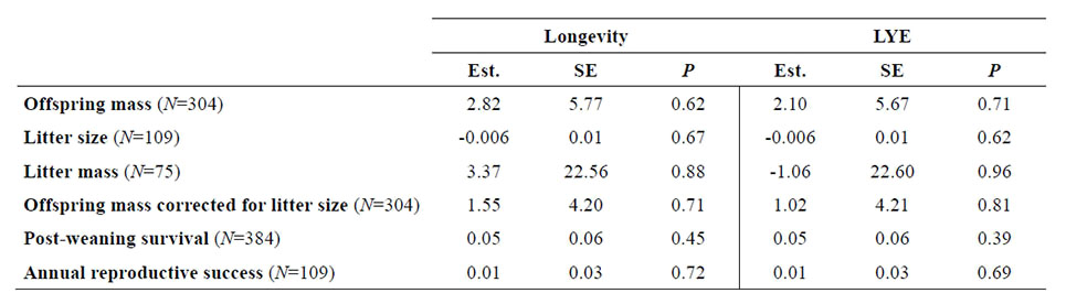
Table C3b. Summary of age-specific models including not statistically significant effects of longevity and last year effect (LYE) on offspring mass, litter size, litter mass, offspring mass corrected for litter size, post-weaning survival and annual reproductive success in female Alpine marmots (Marmota marmota) at La Grande Sassière (French Alps). Est. corresponds to the parameter estimate. SE corresponds to the standard error of the parameter estimate. P corresponds to the p value indicating the statistical significance of the effect of longevity or last year effect (LYE). See Table 3a for details about the model selected for each trait.
Literature cited
Allainé, D., L. Graziani, and J. Coulon. 1998. Postweaning mass gain in juvenile Alpine marmots Marmota marmota.Oecologia 113:370–376.