Ecological Archives E096-003-A1

David T. Milodowski, Simon M. Mudd, and Edward T. A. Mitchard. 2015. Erosion rates as a potential bottom-up control of forest structural characteristics in the Sierra Nevada Mountains. Ecology 96:31–38. http://dx.doi.org/10.1890/14-0649.1

Appendix A. Extended description of methods, and full compilation of results from the statistical analysis.

Field Data

The study area occupies ~83 km², in the western Los Plumas National Forest. The full extent of the original LiDAR survey covers a total of ~208 km²; it extends predominately to the south and southwest. Our reason for limiting the analysis to the northern part of the survey area is that much of the excluded region has either been extensively cleared, or was very heavily damaged during the 2008 fires (either the 2008 Scotch or 2008 Friend/Darnell fires): as we do not have a map of land use history for the area, we are not be able to objectively account for the prevalence of anthropogenic clearing in the southern portions of the LiDAR survey. Since this occurs only in the more low-relief parts of the landscape, this would have obscured the influence of the natural landscape characteristics on the forest properties, which was the primary target of the study. Objective burn intensity maps were obtained from the USFS (accessed from http://www.fs.usda.gov/ on 14/11/2013) enabling us to identify regions that suffered significant fire damage to the structurally dominant vegetation (Miller and Thode 2007, Miller et al. 2009).

During the summers of 2012 and 2013 (post-dating the LiDAR collection by 4–5 years; LiDAR was collected in September 2008 by the National Center for Airborne Laser Mapping (NCALM - http://www.ncalm.org)), we undertook 31 10 m-radius tree inventory plots, recording diameter at breast height (1.3 m), DBH, and species for all trees with DBH>10 cm. Plot positions were determined using a Trimble Geo-XH GPS device, which were post-processed giving positional uncertainties that were typically 20–50 cm. In an earlier study quantifying uncertainty in biomass measurements, Gonzalez et al. (2010) estimated that errors in their measurement of DBH was typically ~3%, which we use as a guide for our uncertainty analysis. All plot locations were located within the footprint of the original LiDAR survey, but not confined to the region used in the study. As much as possible we tried to avoid areas that burned severely in the 2008 fires. Two of the field inventory plots were taken from areas that had been cleared and therefore contained no trees. Our justification for this is that some of the areas within our survey area had also been cleared, thus it was important to include some low biomass plots in our calibration.

Calculating plot biomass and estimating uncertainty

Plot biomass was estimated by calculating the aboveground biomass (AGB) for each tree surveyed using the DBH-based allometric equations (Table A1; Jenkins et al. 2003, Návar 2009, Halpern and Means 2011). We used Nàvar's (2009) equation for Quercus spp. to estimate the biomass of Quercus spp, whilst we used the Jenkins et al. (2003) generalized equations for other tree species. As both the Jenkins et al. (2003) and the Arctostaphylos spp. (Halpern and Means 2011) model estimates had to be back-transformed from log-units, we multiplied this by a correction factor, CF, to account for the back-transformation of the regression error (given by CF=eMSE/2, where MSE is the mean square error) (Baskerville 1972). Uncertainty in the predictions from the back-transformed model, σA, can then be estimated by  (Chave et al. 2004). For the Nàvar (2009) equation, the RMSE was reported in absolute units, so we converted this to a relative RMSE by taking this as a percentage of the mean biomass for the trees used to construct that particular allometric equation, and used this as our estimate on the uncertainty of our predictions. No error estimates were given in the Halpern and Means database, so we assumed a relative error of 30% for Arctostaphylos spp. biomass calculations. Yanai et al. (2010) indicate that using the RMSE leads to an underestimate of the actual uncertainty in individual estimates, but the published equations did not provide the necessary statistics to calculate their preferred uncertainty estimate. Finally it is important to note that interpretation of the RMSE for the Jenkins et al. (2003) equations is complicated by the fact that these equations were derived by fitting "pseudo-data" produced from many different species specific equations, without propagating the uncertainties associated with each individual equation (Jenkins et al. 2003). It is therefore not a direct quantification of the uncertainty in the biomass estimates, but we use it in the absence of an alternative.

Uncertainty in the estimation of plot biomass stems from two sources: measurement error and errors in the prediction from the allometric equation. In order to account for the combined uncertainty in our plot based biomass we developed a Monte Carlo framework to simulate uncertainty in the measurement of DBH and biomass predictions from the allometric equations (Yanai et al. 2010, Gonzalez et al. 2010). Our treatment of errors in the allometric predictions is different to that used for measurement error; errors in measurement of DBH are assumed to be normally distributed and uncorrelated, whereas if there are errors in the allometric model, they are likely to be correlated for other trees of the same species within that plot (Yanai et al. 2010). Therefore, each iteration of the Monte Carlo procedure, errors in DBH are resampled from the probability distribution for each tree, but errors in the allometric equations are sampled once for each iteration, and then the same equation set is used for all trees within the plot. We performed 1000 iterations of our Monte Carlo procedure, and used the mean and standard deviation to estimate the plot biomass and uncertainty respectively.

Calculation of LiDAR-derived biomass and uncertainty

LiDAR has been widely exploited as a tool to quantify spatial variations in AGB across a range of biomes (Lefsky et al. 1999, 2002, Drake et al. 2003, Næsset and Gobakken 2008, Dahlin et al. 2011, Asner et al. 2012, Colgan et al. 2012). We use the mean return height, MRH, defined as the centroid of the canopy return profile for all returns within a 10-m radius, as it combines information on both canopy height and canopy cover into a single variable. This is calibrated against the plot biomass estimates estimated for the 31 field inventory plots surveyed in the field region.

Uncertainty associated with this calibration arises from (i) errors in the plot biomass calculation, discussed above; (ii) positional error (Frazer et al. 2011), from both the original LiDAR georeferencing and GPS measurement error; these errors are additive; (iii) temporal differences between the LiDAR survey and field surveys; (iv) canopy overlap with the edge of the field plot, creating a mismatch between trees identified within the field plots (stem localised) and the corresponding LiDAR point cloud (crown-delimited) (Mascaro et al. 2011). Of these, the latter two are very difficult to quantify, and we do not attempt to here. Positional errors were accounted for using a Monte Carlo sampling procedure; positional uncertainty was represented as a Gaussian distribution, from which we randomly sampled 1000 times, in each of the iterations extracting the MRH for each point cloud sample, and calculating the mean and standard deviations to determine our estimate of plot MRH and its associated uncertainty. Relative errors associated with all these sources, from field plots (Chave et al. 2003, 2004) to calibration of LiDAR-derived metrics (Frazer et al. 2011, Mascaro et al. 2011) are expected to be larger for small plot sizes, and are likely to contribute to significant scatter within our calibration data set. One outlier is excluded from the regression analysis (marked as a hollow symbol in Fig. 2(b) and Fig. A2), as the plot biomass was skewed by the presence of one very large tree (Quercus decurrens, DBH >3 m).

We use a simple linear relationship between plot biomass and MRHas our calibration model for the LiDAR-derived biomass map. Since there are appreciable uncertainties in both calibration variables, we use Standardized Major Axis (SMA) regression to fit the model (Sokal and Rohlf 1995, Warton et al. 2006) using the R package SMATR (Warton et al. 2012). We do not weight the regression, or propagate the estimated uncertainties through other methods such as Monte Carlo methods (e.g., Gonzalez et al. 2010). Our reasoning for this is two-fold: we are not able to fully constrain the uncertainties in each of the variables; the distribution of errors may not be normal for every source of uncertainty. With this in mind, we accept that the absolute biomass values reported in this study have significant uncertainty; however, our calibrated LiDAR model explains 70% of the variance of the plot biomass, with most of the model biomass estimates agreeing with the calibration data set within their estimated error. Thus the uncertainties are unlikely to affect the conclusions drawn from our subsequent geospatial analysis.

Topographic analysis

We investigate the geospatial co-variation in erosion rate and forest characteristics by analyzing the topographic properties of second order drainage basins and their corresponding AGB (Fig. A3). Second order basins represent the catchment area for second order channels, as defined by Strahler stream order: first order channels represent stream reaches stretching from the channel head to the first tributary, at which they become second order channels; second order channel reaches terminate at the confluence with another second (or higher) order channel, and become third order (or higher) channels, etc. From a geomorphic perspective, drainage basins are a fundamental unit in landscape dynamics, as rivers set the lower boundary condition of hillslopes and thus have a first order control on the characteristics of their catchments. The network was extracted by locating channel heads using the DrEICH method developed by Clubb et al. (2014), which has been verified in this landscape (Clubb et al. 2014), and subsequently routing flow via the steepest descent pathway. Extracted basins are shown in Fig. A3. The specific topographic metric that we use is mean basin slope, which provides a first order proxy for erosion rate (Ahnert 1970, Montgomery and Brandon 2002, Hurst et al. 2012). Following Hurst et al. (2012), slope is calculated at each pixel by fitting a six-term polynomial surface to a moving window with a 7-m radius. This filters the effects of small wavelength noise present in high resolution DEMs, which does not reflect the long term evolution of topography.

Downscaling PRISM data

To enable us to account for the influence of climate gradients in our study site, we use the 800-m resolution maps of Mean Annual Precipitation, MAP, and Mean Annual Temperature, MAT, from the PRISM Climate Group at Oregon State University (http://www.prismclimate.org). These maps are produced using the PRISM Parameter-elevation Relationships on Independent Slopes Model) interpolation scheme which incorporates the effects of topography in a physically meaningful way, and has been subject to extensive peer review (e.g., Daly et al. 2002, 2008). Whilst this represents the highest resolution climate data available for our study region, it is based on an 800-m resolution DEM, which is too coarse to account for the microclimatic effects of topography. To address this, we follow the method outlined by Chorover et al. (2011) to downscale this climate data (see also Pelletier et al. 2013). Both MAT and MAP were resampled to 10-m resolution using spline interpolation, and then MAT was modified to account for the microclimatic effects of local topography on incoming solar radiation (Yang et al. 2007).

Basin Lithology

The bedrock geology classification for each catchment was determined by selecting the dominant (i.e., >50%) lithology present in the basin, as determined from the USGS geological map of California (Fig. A3; from Ludington et al. 2005). To simplify the analysis of lithology, we used a binary classification splitting the basins into basins that are predominately underlain by granodiorite, and those underlain by other lithologies.

Statistical analysis of controls on AGB

We use a General Linear Model framework to explore the extent to which mean basin slope, basin-averaged MAP and MAT, and bedrock lithology can explain the variance in the AGB for the second order basins extracted for the landscape, using the statistical computing environment R (R Core Team 2013). In total, 16 different models were tested, the results of which are presented in Tables A2 and A3. In order to account for the effects of the 2008 Scotch Fire, we focused on a sub-set of catchments, in which the biomass map was first filtered to remove parts of the forest that were categorized as suffering moderate/high severity fire damage in the USFS burn severity map, and any basins for which >50% of their area was affected were removed from the sample. The exceptions are Model 1 and Model 2, which use the full data set. Since the fire only affected granodiorite catchments, we only tested the impact of lithology in the filtered data set, as otherwise the results would very likely be biased by the impact of the fire damage on the levels of AGB in affected catchments.

Table A1. Allometric equations used to estimate biomass of individual trees in the field inventory plots.

Notes: Abbreviations: DBH: Diameter at Breast Height (1.3m), in cm; DBA: Diameter at Base, in cm; AGB:Aboveground Biomass, in kg.

Table A2. The results from 16 different GLM analyzes exploring the controls on the variation of mean AGB for all second order drainage basins within the study region.

Notes: †full data set; for all other models, the analysis excluded areas that suffered moderate-severe canopy disturbance during the 2008 Scotch fire, and completely excludes basins for which the affected area accounted for >50% of the total catchment area. Abbreviations: MBS = mean basin slope; MAP = mean annual precipitation; MAT = mean annual temperature. Lithology factor varies according to dominant bedrock lithology: 1 = granodiorite; 0 = meta-volcanics

Table A3. Full results from the GLM analysis exploring controls on the variation of mean AGB for all 2nd order drainage basins. This includes full suite of models explored including and excluding lithology as a factor.

Table A3. (continued)

Notes: Models numbered according to Table A2. Abbreviations: MBS = mean basin slope; MAP = mean annual precipitation; MAT = mean annual temperature. Lithology factor varies according to dominant bedrock lithology: 1 = granodiorite; 0 = meta-volcanics. Significance codes: *** p < 0.001; ** p < 0.01; * p < 0.05; p < 0.01.

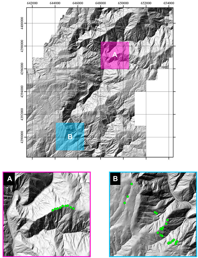
Fig. A1. A shaded relief map indicating the locations of the field inventory plots (green), from which we calculated plot biomass to calibrate the LiDAR-derived biomass estimates. The coordinate system is UTM Zone 10N.

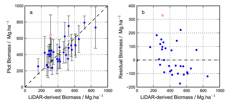
Fig. A2. (a) Comparison of plot-based biomass and LiDAR-derived biomass estimates. (b) Residual plot for the regression model. In both cases the outlier (marked by the hollow symbol) was excluded from the regression (see text for discussion).

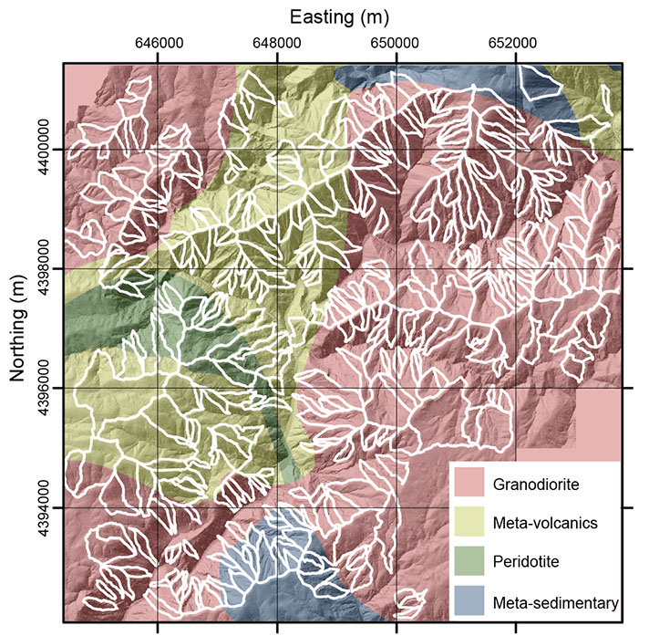
Fig. A3. A geological map of the study region (Ludington et al. 2005), with the outlines of second order drainage basins analysed in this study outlined in white. The coordinate system is UTM Zone 10N.

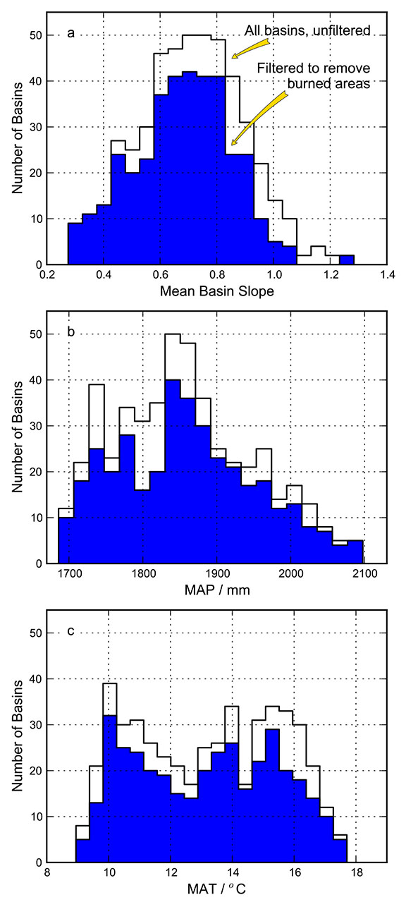
Fig. A4. Histograms of the explanatory variables: (a) Mean basin slope; (b) MAP; (c) MAT. The population distribution of both the full, unfiltered dataset of basins greater than 20,000 m² (black outline) and filtered data set of basins (blue, filled), in which areas badly affected by the 2008 fire are removed, are shown.

Literature cited

Ahnert, F. 1970 Functional Relationships Between Denudation, Relief, and Uplift in Large Mid-Latitude Drainage Basins. American Journal of Science 268:243–263.

Asner, G. P., J. Mascaro, H. C. Muller-Landau, G. Vieilledent, R. Vaudry, M. Rasamoelina, J. S. Hall, and M. van Breugel. 2012. A universal airborne LiDAR approach for tropical forest carbon mapping. Oecologia 168:1147–1160.

Baskerville, G. L. 1972. Use of Logarithmic Regression in the Estimation of Plant Biomass. Canadian Journal of Forest Research 2:49–53.

Chave, J., R. Condit, S. Aguilar, A. Hernandez, S. Lao, and R. Perez. 2004. Error propagation and scaling for tropical forest biomass estimates. Philosophical Transactions of the Royal Society B: Biological Sciences 359:409–420.

Chave, J., R. Condit, S. Lao, J. P. Caspersen, R. B. Foster, and S. P. Hubbell. 2003. Spatial and temporal variation of biomass in a tropical forest: results from a large census plot in Panama. Journal of Ecology 91:240–252.

Chorover, J., P. A. Troch, C. Rasmussen, P. D. Brooks, J. D. Pelletier, D. D. Breshars, T. E. Huxman, S. A. Kurc, K. A. Lohse, J. C. McIntosh, T. Meixner, M. G. Schaap, M. E. Litvak, J. Perdrial, A. Harpold, and M. Durcik. 2011. How Water, Carbon, and Energy Drive Critical Zone Evolution: The Jemez–Santa Catalina Critical Zone Observatory. Vadose Zone Journal 10:884–899.

Clubb, F. J., S. M. Mudd, D. T. Milodowski, M. D. Hurst, and L. J. Slater. 2014. Objective extraction of channel heads from high-resolution topographic data. Water Resources Research 50:4283–4304.

Colgan, M. S., G. P. Asner, S. R. Levick, R. E. Martin, and O. A. Chadwick. 2012. Topo-edaphic controls over woody plant biomass in South African savannas. Biogeosciences 9:1809–1821.

Dahlin, K. M., G. P. Asner, and C. B. Field. 2011. Environmental filtering and land-use history drive patterns in biomass accumulation in a mediterranean-type landscape. Ecological Applications 22:104–118.

Daly, C., W. P. Gibson, G. H. Taylor, G. L. Johnson, and P. Pasteris. 2002. A knowledge-based approach to the statistical mapping of climate. Climate research 22:99–113.

Daly, C., M. Halbleib, J. I. Smith, W. P. Gibson, M. K. Doggett, G. H. Taylor, J. Curtis, and P. P. Pasteris. 2008. Physiographically sensitive mapping of climatological temperature and precipitation across the conterminous United States. International Journal of Climatology 28:2031–2064.

Drake, J. B., R. G. Knox, R. O. Dubayah, D. B. Clark, R. Condit, J. B. Blair, and M. Hofton. 2003. Above-ground biomass estimation in closed canopy Neotropical forests using lidar remote sensing: factors affecting the generality of relationships. Global Ecology and Biogeography 12:147–159.

Frazer, G. W., S. Magnussen, M. A. Wulder, and K. O. Niemann. 2011. Simulated impact of sample plot size and co-registration error on the accuracy and uncertainty of LiDAR-derived estimates of forest stand biomass. Remote Sensing of Environment 115:636–649.

Gonzalez, P., G. P. Asner, J. J. Battles, M. A. Lefsky, K. M. Waring, and M. Palace. 2010. Forest carbon densities and uncertainties from Lidar, QuickBird, and field measurements in California. Remote Sensing of Environment 114:1561–1575.

Halpern, C., and J. Means. 2011. Pacific Northwest Plant Biomass Component Equation Library. Database. http://andrewsforest.oregonstate.edu/data/abstract.cfm?dbcode=TP072.

Hurst, M. D., S. M. Mudd, R. Walcott, M. Attal, and K. Yoo. 2012. Using hilltop curvature to derive the spatial distribution of erosion rates. Journal of Geophysical Research-Earth Surface 117.

Jenkins, J. C., D. C. Chojnacky, L. S. Heath, and R. A. Birdsey. 2003. National-scale biomass estimators for United States tree species. Forest Science 49:12–35.

Lefsky, M. A., W. B. Cohen, D. J. Harding, G. G. Parker, S. A. Acker, and S. T. Gower. 2002. Lidar remote sensing of above-ground biomass in three biomes. Global Ecology and Biogeography 11:393–399.

Lefsky, M. A., D. Harding, W. Cohen, G. Parker, and H. Shugart. 1999. Surface Lidar Remote Sensing of Basal Area and Biomass in Deciduous Forests of Eastern Maryland, USA. Remote Sensing of Environment 67:83–98.

Ludington, S., B. C. Moring, R. J. Miller, K. S. Flynn, P. A. Stone, and D. R. Bedford. 2005. Preliminary integrated databases for the United States - Western States: California, Nevada, Arizona, and Washington. U.S. Geological Survey, Reston, Virginia, USA.

Mascaro, J., M. Detto, G. P. Asner, and H. C. Muller-Landau. 2011. Evaluating uncertainty in mapping forest carbon with airborne LiDAR. Remote Sensing of Environment 115:3770–3774.

Miller, J. D., E. E. Knapp, C. H. Key, C. N. Skinner, C. J. Isbell, R. M. Creasy, and J. W. Sherlock. 2009. Calibration and validation of the relative differenced Normalized Burn Ratio (RdNBR) to three measures of fire severity in the Sierra Nevada and Klamath Mountains, California, USA. Remote Sensing of Environment 113:645–656.

Miller, J. D., and A. E. Thode. 2007. Quantifying burn severity in a heterogeneous landscape with a relative version of the delta Normalized Burn Ratio (dNBR). Remote Sensing of Environment 109:66–80.

Montgomery, D., and M. Brandon. 2002. Topographic controls on erosion rates in tectonically active mountain ranges. Earth and Planetary Science Letters 201:481–489.

Næsset, E., and T. Gobakken. 2008. Estimation of above- and below-ground biomass across regions of the boreal forest zone using airborne laser. Remote Sensing of Environment 112:3079–3090.

Návar, J. 2009. Allometric equations for tree species and carbon stocks for forests of northwestern Mexico. Forest Ecology and Management 257:427–434.

Pelletier, J. D., G. A. Barron-Gafford, D. D. Breshears, P. D. Brooks, J. Chorover, M. Durcik, C. J. Harman, T. E. Huxman, K. A. Lohse, R. Lybrand, T. Meixner, J. C. McIntosh, S. A. Papuga, C. Rasmussen, M. Schaap, T. L. Swetnam, and P. A. Troch. 2013. Coevolution of nonlinear trends in vegetation, soils, and topography with elevation and slope aspect: A case study in the sky islands of southern Arizona. Journal of Geophysical Research: Earth Surface 118:741–758.

R Core Team. 2013. R: A language and environment for statistical computing. R Foundation for Statistical Computing, Vienna, Austria.

Sokal, R. R., and F. J. Rohlf. 1995. Biometry: the principles and practice of statistics in biological sciences. WH Freeman and Company, New York, USA.

Warton, D. I., R. A. Duursma, D. S. Falster, and S. Taskinen. 2012. smatr 3– an R package for estimation and inference about allometric lines. Methods in Ecology and Evolution 3:257–259.

Warton, D. I., I. J. Wright, D. S. Falster, and M. Westoby. 2006. Bivariate line-fitting methods for allometry. Biological Reviews 81:259–291.

Yanai, R. D., J. J. Battles, A. D. Richardson, C. A. Blodgett, D. M. Wood, and E. B. Rastetter. 2010. Estimating Uncertainty in Ecosystem Budget Calculations. Ecosystems 13:239–248.

Yang, X., G. Tang, C. Xiao, and F. Deng. 2007. Terrain revised model for air temperature in mountainous area based on DEMs. Journal of Geographical Sciences 17:399–408.

[Back to E096-003]