Ecological Archives E095-232-D1

Laura Kirwan, John Connolly, Caroline Brophy, Ole Baadshaug, Gilles Belanger, Alistair Black, Tim Carnus, Rosemary Collins, Jure Čop, Ignacio Delgado, Alex De Vliegher, Anjo Elgersma, Bodil Frankow-Lindberg, Piotr Golinski, Philippe Grieu, Anne-Maj Gustavsson, Áslaug Helgadóttir, Mats Höglind, Olivier Huguenin-Elie, Marit Jørgensen, Žydre Kadžiulienė, Tor Lunnan, Andreas Lüscher, Päivi Kurki, Claudio Porqueddu, M.-Teresa Sebastia, Ulrich Thumm, David Walmsley, and John Finn.. 2014. The Agrodiversity Experiment: three years of data from a multisite study in intensively managed grasslands. Ecology 95:2680. http://dx.doi.org/10.1890/14-0170.1

Metadata

Class I. Data set descriptors

A. Data set identity: The Agrodiversity Experiment: three years of data from a multisite plant diversity experiment in intensively managed grasslands.

B. Data set identification code: site_info.csv biomass.csv forage_quality.csv climate.csv soils.csv

C. Data set description

Abstract: Intensively managed grasslands are globally prominent ecosystems. We investigated whether experimental increases in plant diversity in intensively managed grassland communities can increase their resource use efficiency. This work consisted of a coordinated, continental-scale 33-site experiment. The core design was 30 plots, representing 15 grassland communities at two seeding densities. The 15 communities were comprised of four monocultures (two grasses and two legumes) and 11 four-species mixtures that varied in the relative abundance of the four species at sowing. There were 1028 plots in the core experiment, with another 572 plots sown for additional treatments. Sites agreed a protocol and employed the same experimental methods with certain plot management factors, such as seeding rates and number of cuts, determined by local practice. The four species used at a site depended on geographical location, but the species were chosen according to four functional traits: a fast-establishing grass, a slow-establishing persistent grass, a fast-establishing legume, and a slow-establishing persistent legume. As the objective was to maximize yield for intensive grassland production, the species chosen were all high-yielding agronomic species. The data set contains species-specific biomass measurements (yield per species and of weeds) for all harvests for up to four years at 33 sites. Samples of harvested vegetation were also analyzed for forage quality at 26 sites. Analyses showed that the yield of the mixtures exceeded that of the average monoculture in >97% of comparisons. Mixture biomass also exceeded that of the best monoculture (transgressive overyielding) at about 60% of sites. There was also a positive relationship between the diversity of the communities and aboveground biomass that was consistent across sites and persisted for three years. Weed invasion in mixtures was very much less than that in monocultures.

These data should be of interest to ecologists studying relationships between diversity and ecosystem function and to agronomists interested in sustainable intensification. The large spatial scale of the sites provides opportunity for analyses across spatial (and temporal) scales. The database can also complement existing databases and meta-analyses on biodiversity–ecosystem function relationships in natural communities by focusing on those same relationships within intensively managed agricultural grasslands.

D. Key words: agricultural grasslands; biodiversity; ecosystem function; forage quality; mixtures; monocultures; overyielding; plant community; species biomass; yield.

E. Authors:

Laura Kirwan,^1,25 John Connolly,² Caroline Brophy,³ Ole Baadshaug,⁴ Gilles Belanger,⁵ Alistair Black,⁶ Tim Carnus,^2,7 Rosemary Collins,⁸ Jure Čop,⁹ Ignacio Delgado,¹⁰ Alex De Vliegher,¹¹ Anjo Elgersma,¹² Bodil Frankow-Lindberg,¹³ Piotr Golinski,¹⁴ Philippe Grieu,¹⁵ Anne-Maj Gustavsson,¹⁶ Áslaug Helgadóttir,¹⁷ Mats Höglind,¹⁸ Olivier Huguenin-Elie,¹⁹ Marit Jørgensen,¹⁸ Žydrė Kadžiulienė,²⁰ Tor Lunnan,¹⁸ Andreas Lüscher,¹⁹ PÄivi Kurki,²¹ Claudio Porqueddu,²² M.-Teresa Sebastia,²³ Ulrich Thumm,²⁴ David Walmsley,^1,7 and John Finn⁷

1 Waterford Institute of Technology, Cork Road, Waterford, Ireland

2 School of Mathematical Sciences, University College Dublin, Dublin 4, Ireland

3 Department of Mathematics and Statistics, National University of Ireland Maynooth, Maynooth, County Kildare, Ireland

4 Department of Plant Sciences, Norwegian University of Life Sciences, P.O. Box 5003, N-1432 Ås, Norway

5 Agriculture and Agri-Food Canada, 2560, Hochelaga Blvd, Québec, Québec G1V 2J3, Canada

6 Faculty of Agriculture and Life Sciences, PO Box 85084, Lincoln University, Lincoln 7647, Christchurch, New Zealand

7 Teagasc, Environment Research Centre, Johnstown Castle, Wexford, Ireland

8 Aberystwyth University, IBERS, Plas Gogerddan, Aberystwyth SY23 3EE, Wales, UK

9 Biotechnical Faculty, University of Ljubljana, Jamnikarjeva 101, SI-1000 Ljubljana, Slovenia

10 CITA-DGA, Av. Montañana 930, 50059 Zaragoza, Spain

11 ILVO, Plant Sciences Unit, Crop Husbandry and Environment, B. Van Gansberghelaan 109, 9820 Merelbeke, Belgium

12 Plant Sciences Group, Wageningen University, PO Box 16, 6700 AA Wageningen, The Netherlands

13 Swedish University of Agricultural Sciences, Department of Crop Production Ecology, Box 7043, SE-750 07 Uppsala, Sweden

14 Department of Grassland and Natural Landscape Sciences, Poznan University of Life Sciences, Wojska Polskiego 38/42, 60-627 Poznan, Poland

15 University of Toulouse; UMR AGIR, INP-ENSAT, F-31326 Castanet Tolosan, France

16 Swedish University of Agricultural Sciences, Department of Agricultural Research for Northern Sweden, SE-901 83 Umeå, Sweden

17 Agricultural University of Iceland, Árleyni 22, IS-112 Reykjavík, Iceland

18 Bioforsk, Norwegian Institute for Agricultural and Environmental Research, Frederik A. Dahls vei 20, N-1430 ÅS

19 Agroscope Institute for Sustainability Sciences ISS, Reckenholzstrasse 191, 8046 Zurich, Switzerland

20 Institute of Agriculture, Lithuanian Research Centre for Agriculture and Forestry, Akademija, LT-58344, Kedainiai, Lithuania

21 MTT Agrifood Research Finland, Plant Production Research Lönnrotinkatu 5, FI - 50100 Mikkeli, Finland

22 CNR-ISPAAM, Traversa la Crucca 3, località Baldinca, 07100 Sassari, Italy

23 Centre Tecnologic Forestal de Catalunya, Ctra Sant Llorenç km 2, 25280 Solsona, Spain

24 University of Hohenheim, Department  of Crop Science, 70593 Stuttgart, Germany

25 Corresponding author. E-mail: [email protected]

Class II. Research origin descriptors

The Agrodiversity experiment was a coordinated continental-scale field experiment. The coordination of the network was supported by EU COST Action 852: Quality Legume-Based Forage Systems for Contrasting Environments. Each of the 33 participating sites established at least 30 plots using the same experiment design and managed the plots according to an agreed protocol. The design of the experiment consisted of a common set of 30 plots across all sites, with additional optional plots for applying treatments. Aboveground biomass was measured at the common set of 30 plots for all harvests at all sites. Forage quality measurements were undertaken at 26 sites. Additional treatments were voluntarily undertaken by various sites. The treatments applied varied across sites and included increased genetic diversity in species, different levels of nitrogen fertilizer and different levels of cutting intensity.

The network did not have a central funding source to cover the costs of running the experiment, thus participating sites each secured funding to cover the costs incurred at their own site; COST852 provided funding for regular meetings and for scientific networking between partners. The collation of this database was supported by the Irish Research Council for Science, Engineering and Technology through a research fellowship to L. Kirwan, with additional support from Science Foundation Ireland Research Frontiers Programme (09/RFP/EOB2546).

The email addresses of people that have contributed to the data are included in the file site_info.csv. Those in the best position to answer questions concerning the data are Laura Kirwan ([email protected]) and Caroline Brophy ([email protected]); those in the best position to answer questions about experimental protocol are Andreas Lüscher ([email protected]) and Maria-Teresa Sebastià ([email protected]); those in the best position to answer questions concerning the experimental design are John Connolly ([email protected]) and Laura Kirwan ([email protected]).

Introduction

Ecological research on the relationship between plant diversity and ecosystem function generally shows that reductions in plant diversity of randomly-assembled communities reduce the yield of aboveground biomass (Cardinale et al. 2007). Mechanisms that underpin these relationships are attributed to improved utilization of resources in total niche space (niche differentiation), positive interspecific interactions, and selection effects (Hooper et al. 2005). Most such experiments (as reviewed in Cardinale et al. 2007) study the effects of reductions in plant richness from relatively species-rich communities and in low-nutrient systems. In contrast, conventional agriculture in many areas maximises forage yield by planting monocultures of grasses and applying large quantities of nitrogen fertilizer, and has associated negative environmental impacts. We are interested in the role of multi-species agricultural mixtures in improving the resource use efficiency of agricultural grassland systems. If the same diversity-function mechanisms and relationships prevail in simple multi-species plant communities and under higher applications of nutrients, then increased plant diversity in species-poor agricultural systems would be expected to improve their resource-efficient provision of forage and other ecosystem services. For generality and relevance to agricultural practice, investigations of multi-species mixtures need to be conducted at multiple sites, and require comparison against the best-performing component monoculture species (or the prevailing conventional system).

The species composition of multi-species mixtures can be strategically designed to include traits that maximize complementarity and interspecific interactions to improve resource utilization and yield of aboveground biomass. A classic example is the combination of grass and legume species to exploit the ability of legumes to fix atmospheric nitrogen and thereby reduce reliance on application of chemical fertilizers (Nyfeler et al. 2011). However, other traits are also likely to be relevant, but are not usually explicitly tested in multi-species experiments conducted across multiple sites, years and mixture types. Here we test a temporal development trait. Fast-establishing species exhibit fast germination and growth, thereby providing adequate cover of soil and high biomass yields in the first and second year after sowing. These species often lack persistency. Slow-establishing, but persistent species exhibit slower germination and growth rate during establishment, but in the long run are highly competitive, therefore increasing in cover and biomass yields over initial years and constituting the majority of yield in the third and fourth production year and thereafter.

In this data paper, we present data from the Agrodiversity experiment, a co-ordinated continental-scale field experiment across 33 sites that was used to compare the biomass yield of monocultures and four-species mixtures (designed on the basis of specific traits) associated with intensively managed agricultural grassland systems. We addressed the following main questions (modified from Finn et al. 2013):

1. Were there yield benefits (overyielding) from diversity and, if so, did the benefits persist over three years and across sites?
2. Were the yield benefits sufficiently large for transgressive overyielding to occur?
3. Did the benefits of diversity occur and persist across the range of mixture communities used in this experiment?
4. Did both the functional traits of nitrogen acquisition and temporal development contribute to the diversity effect (the excess of mixture performance over that of the monoculture performances of component species)?
5. What were the differences in resistance to weed invasion, nutrient dynamics and forage quality among the different plant communities?
6. What were the factors affecting the stability of species composition?

Recent analyses of some of these data quantified the relationships between community diversity and aboveground biomass (Kirwan et al. 2007, Finn et al. 2013). We showed that aboveground biomass of the mixtures exceeded that of the average monoculture in >97% of comparisons, and mixture biomass also exceeded that of the best monoculture (transgressive overyielding) at about 60% of sites (Finn et al. 2013). There was also a positive relationship between the evenness of the communities and aboveground biomass that was consistent across sites (Kirwan et al. 2007) and persisted for three years (Finn et al. 2013). In an analysis across six sites, positive yield effects were not accompanied by a reduction in herbage digestibility and crude protein concentration (Sturludóttir et al. 2013).

Ultimately, we hope that further analyses of this data set will promote understanding about (a) the design of multi-species mixtures for application in more resource-efficient agricultural systems and (b) how the diversity (composition, richness and relative abundance) of plant communities influences the delivery of ecosystem processes across spatial and temporal scales.

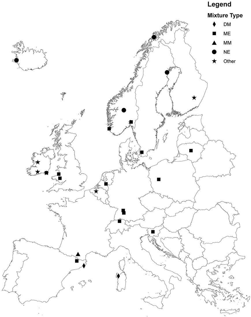
Fig. 1. Map of site locations in Europe. Geographical locations of the sites are indicated for the Mid-European (ME), North-European (NE), Dry-Mediterranean (DM), Moist-Mediterranean (MM) and Other species groups. Note that there is an additional site in Canada. Coordinates for each site are contained in site_info.csv

Methods

Description of the study area and experimental design:

This was a coordinated multi-site experiment in which sites a covered a broad geographical area (Fig. 1). Details of site coordinates, altitude, species and varieties used, plot management and any treatments applied are in site_info.csv.

Design of the core experiment:

The species compositions of experimental plots were selected using a simplex design for mixtures experiments (Cornell [2002] Table 1). At each site, four species were chosen according to four functional traits: a fast-establishing grass (G1), a slow-establishing persistent grass (G2), a fast-establishing legume (L1) and a slow-establishing persistent legume (L2). The species selected by individual sites are detailed in site_info.csv. The species chosen generally fell into four groups according to geographical location: Mid-European (18 sites), North-European (6 sites), Dry Mediterranean (2 sites) and Moist Mediterranean (1 site), with seven sites selecting site-specific species (Other). As the objective was to maximise yield of highly digestible forage from intensive grasslands, the chosen species were all high-yielding agronomic species.

The main treatment consisted of a core set of 30 plots, representing fifteen grassland communities at two levels of seed density. At each site, the four species were sown in monoculture, with sowing rates determined by each site according to local practice. The sowing rates of the four species were systematically varied to produce eleven mixture communities. These fifteen communities were repeated at low and high levels of seeding density ('high' was represented by the standard seeding rate of a monoculture species at a site, with 'low' being 60% of the high seeding rate). Relative proportions of species in a mixture were manipulated by varying seeding rates of the four species at sowing, and resulted in four planned levels of evenness in the design (Table 1). This design resulted in a core set of 30 experimental plots per site (arranged in a completely randomized design).

The species richness of the communities was either one (monocultures) or four (mixtures). However within the four-species mixtures, the level of evenness was manipulated. The levels of evenness (E) were calculated using the formula

,

where s is the maximum number of species in a community (s = 4 for this experiment), and P_i is the sown relative abundance of the ith species (see Kirwan et al. 2007). This lies between 0 for monocultures and 1 for a community in which all species are represented in equal proportions.

Two sites (45 and 46) were not part of the initial network and did not use this core design. They used a variation of the design. The data from these sites is included because there is high overlap in communities with those in the core design. The same plot number is given to design points (community type) at sites 45 and 46 that are the same as those in the core design. This facilitates similar analyses and inclusion in meta-analysis. Sites 45 and 46 included two-species mixtures, whereas the core design does not.

Note on replication: Within a site, the design is not replicated. The design of the experiment was optimized for good coverage of species composition in order to facilitate the use of a response surface regression approach. In regression analyses, one usually does not require replication and residual variation is estimated from the lack of fit of individual points to the regression model selected. However, the use of two seeding densities adds effective replication for mixture communities. The large number of individual experiments across different sites generally adds a very high level of statistical power to the overall experimental design.

Additional treatments:

Additional plots were sown at 22 sites to facilitate the assessment of an experimental treatment. The most commonly applied treatment was a wide genetic base (WGB) treatment, applied at ten sites. A nitrogen fertilizer application treatment was applied at eight sites.

A treatment to investigate genetic diversity was applied at ten sites. At these sites, the treatment plots were sown with legume species with increased intraspecific genetic diversity. The single varieties of white and red clover selected at each site were compared with a wide genetic base (WGB) treatment that consisted of composite populations of white and red clover that were each constructed from commercial varieties plus unselected material obtained from germplasm collections. Different WGB composite populations were constructed for white and red clover species for the ME and NE regions. The seed material for the WGB treatment was supplied to the participating sites and the populations supplied depended on whether the site had used the ME or NE species group for the core experiment. Further details on the composite populations and an analysis of the temporal change in genetic diversity at three sites was published in Collins et al. (2012).

At eight sites, an additional nitrogen fertilizer application level was tested. Details of the amounts of N applied at core and treatment plots are detailed in site_info.csv. The treatments applied at the other sites were cutting frequency, different legume species, and local varieties of the species.

Table 1. Description of experiment design. G1, G2, L1, and L2 represent the sowing proportions of the four species. E is the planned evenness of the community. Density is the sowing density (low is 60% of high) and is determined by each site according to local practice. Type indicates whether the design point is part of the core design, or an additional optional treatment. The core 30 plots make up the main experiment (shaded). The additional 18 treatment plots were established at 18 sites and the treatments applied are detailed in site_info.csv. Plots 49–68 are additional plots that were sown at sites 45 and 46. # Sites indicates the number of sites in which a particular community was sown.

Management protocol:

Plots were not grazed. The number of cuts per annum and fertilizer application levels were determined by local practice at individual sites. See Site_info.csv for details on management practices employed at each site.

The plots were not weeded and there was generally no herbicide application. However, some targeted weeding was required in some sites during the establishment phase. See Site_info.csv for details on weeding in the establishment year. Margins between plots were sprayed to prevent stoloniferous ingression from neighboring plots.

Year 1 was defined as the first complete year after sowing. Some sites took cleaning cuts in the year of establishment (prior to year 1), but data is not recorded for these cuts. See Site_info.csv for details on cleaning cuts.

Response variables:

The response variables included in the database are total biomass, biomass of the five harvest fractions (G1, G2, L1, L2, weed) and measurements of forage quality. Analyses of total plot biomass and biomass of weed species have been published in Kirwan et al. (2007), Lüscher et al. (2008), Frankow-Lindberg et al. (2009), Nyfeler et al. (2009, 2011) and Finn et al. (2013). An analysis of forage quality at 4 sites was published in Sturludóttir et al. (2013).

Total Biomass per plot

For each plot, biomass of aboveground vegetation was measured at each harvest. This was done by cutting the whole plot and determining the fresh weight of the 'whole plant material'. A subsample of this material was taken, its fresh weight determined and the material dried at 65°C to constant weight. From the dry weight of the sample the percentage dry matter was calculated. From this, the total dry matter yield for the plot (DM/m²) was calculated from the fresh mass of the 'whole plant material'.

Biomass of the five harvest fractions (G1, G2, L1, L2, weed)

Biomass separation was done by one of the following two methods: (see Site_info.csv for method selected for each site). The harvests at which separate determination was carried out are given in biomass.csv.

1. Fixed quadrat: A fixed 50 × 50 cm² quadrat was established in the middle of each plot and cut (to the standard height) separately from the rest of the plot. The plant material in the quadrat was separated into the five basic fractions: G1, G2, L1, L2, weed and dried at 65°C to constant weight. The five fractions were weighed separately.
2. Grabbed sample: Several samples of biomass were taken by hand from the plot and mixed. A sub-sample of the mixture of minimum size 200 g fresh mass was taken. The sub-sample material was separated into the five fractions: G1, G2, L1, L2, weed, dried at 65°C to constant weight and each fraction weighed.

Note on indigenous plants of experimental species (G1, G2, L1, L2): In the mixture plots indigenous (not sown) G1, G2, L1, and L2 plants cannot be separated from the sown plants of these species and so do not form part of the weed fraction. However, in each monoculture plot, indigenous plants of the other three species are included in weed.

Forage quality

The primary forage quality analysis was carried out at the Christian-Albrechts-Universität Kiel, Kiel, Germany. Additional analysis for four North European sites was carried out at Agriculture and Agrifood Canada at Levis, Canada. This analysis of samples from the North-European sites has been published in Sturludóttir et al. (2013). In addition, N concentration of bulk samples was locally analyzed by 21 sites. Forage quality data is given in forage_quality.csv. Measurements are coded _K, _C or _L to indicate whether samples were analysed at Kiel, Canada or local laboratories.

Kiel analysis: Bulk samples (not separated into component species) were analysed for 17 sites. At seven of the sites, all plots were analyzed. At 10 sites, samples were analyzed for 18 out of the 30 experimental plots (the 12 plots in the design co-dominated by two species were omitted). Separation of the forage into the five fractions was also considered for those particularly interested in the forage quality of the different functional groups. Separated samples were analyzed for eight sites. Sample material of at least 5 g per sample was prepared by drying to a constant weight at 65°C and then grinding to pass through a sieve of 1-mm mesh size. Near-infrared spectroscopy (NIRS) analysis was carried out to determine the dry matter percentage of nitrogen concentration (N), ADF (acid detergent fibre) NDF (neutral detergent fibre), ELOS (enzymatic soluble organic dry matter), and ash which represents the mineral content of the sample.

Canadian analysis: Bulk samples were analyzed for four sites. Samples were analysed for all plots. Samples were dried and ground and then analyzed using NIRS (FOSS NIRsystems 6500, Silver Spring, MD) to determine nitrogen concentration (N), acid detergent fiber (ADF), neutral detergent fiber (NDF), in vitro true digestibility (IVTD) and in vitro cell wall digestibility (IVCWD). The latter was calculated using the following equation: IVCWD = 1000 - [(1000 – IVTD)/(NDF/1000)].

Site description variables:

Climate data

Each site provided daily climate data for the duration of their experiment. Where possible, the climate data series begins on the sowing date of the experiment at each site. The variables recorded were precipitation (mm per day), minimum daily air temperature (°C), mean daily air temperature (°C) and maximum daily air temperature (°C). The climate data is contained in climate.csv.

Soil analysis

The soil analysis was carried out at Centre Tecnològic Forestal de Catalunya, Solsona, Spain. Composite soil samples were formed by combining samples from four plots. In each sampled plot a soil volume of 5 × 5 cm² per 15 cm depth was taken in a systematic manner, as follows. To avoid soil contamination by litter, the first 0.5 cm of litter-soil was removed. The composite sample was dried (temperature between 20 and 40ºC) over two or three days. The soil aggregates were gently ground and passed through a 2-mm sieve, discarding the fraction >2 mm. A 300 g subsample was sent to the laboratory for analysis. The percentage of sand, silt, fine silt, and clay were measured and the soil type classified. In addition, percent organic matter, soil carbonates, soil electrical conductivity and soil pH were measured, along with the concentrations of calcium, potassium, nitrate, magnesium, sodium, and phosphorus.

Data set description

Data from individual sites was recorded in standardized data recording spreadsheets and then collated into a central database. Data was checked using numerical and graphical summary methods. Data range was checked for each variable and pivot tables were used to check counts of measurements. The datasets were manipulated and merged using the SORT, MERGE, and DATA procedures in SAS 9.1 (SAS Institute Inc., Cary, NC, USA).

Descriptions and units of measurement for the columns of data are presented in the tables below. Site-level information is contained in the comma-separated-value data files named site_info.csv, climate.csv and soils.csv. Data relating to plot-level measurements are contained in the comma-separated-value data files named biomass.csv and forage_quality.csv. Note that in all files missing data values are represented by empty cells.

Column numbers, variable names and variable descriptions for file: site_info.csv

Column numbers, variable names, and variable descriptions for file: climate.csv

Column numbers, variable names, and variable descriptions for file: soils.csv

Column numbers, variable names, and variable descriptions for file: biomass.csv

Column numbers, variable names, and variable descriptions for file: forage_quality.csv

DATA-USE POLICY

The data presented here are publicly available. Those wishing to publish results from this data set should read this metadata document. The data set should be cited as: Kirwan et al. 2014. The Agrodiversity Experiment: three years of data from a multisite plant diversity experiment in intensively managed grasslands. Ecology xx:xxx.

Three papers are currently in preparation, focusing on (a) the effect of diversity on the contribution of weed species to biomass yield, (b) changes in the relative abundances of the mixtures, and (c) grassland biodiversity effects across an environmental gradient.

Literature cited

Cardinale, B. J., J. P. Wright, M. W. Cadotte, I. T. Carroll, A. Hector, D. S. Srivastava, M. Loreau, and J. J. Weis. 2007. Impacts of plant diversity on biomass production increase through time because of species complementarity. Proceedings of the National Academy of Sciences of the United States of America 104:18123–18128.

Collins, R. P., A. Helgadóttir, B. E. Frankow-Lindberg, L. Skøt, C. Jones, and K. P. Skøt. 2012. Temporal changes in population genetic diversity and structure in red and white clover grown in three contrasting environments in northern Europe. 2012. Annals of Botany 110(6):1341–1350.

Connolly, J., J. A. Finn, A. D. Black, L. Kirwan, C. Brophy, and A. Lüscher. 2009. Effects of multi-species swards on biomass production and weed invasion at three Irish sites. Irish Journal of Agricultural and Food Research. 48:243–260.

Cornell, J. A. 2002. Experiment with Mixtures: Designs, Models, and the Analysis of Mixture Data, Third Edition, John Wiley & Sons, Inc., USA.

Finn, J. A., L. Kirwan, J. Connolly, M. T. Sebastià, A. Helgadottir, O. H. Baadshaug, G. Bélanger, A. Black, C. Brophy, R. P. Collins, J. Čop, S. Dalmannsdóttir, I. Delgado,A. Elgersma, M. Fothergill, B. E. Frankow-Lindberg, A. Ghesquiere, B. Golinska, P. Golinski, P. Grieu, A. -M. Gustavsson, M. Höglind, O. Huguenin-Elie, M. Jørgensen, Z. Kadziuliene, P. Kurki, R. Llurba, T. Lunnan, C. Porqueddu, M. Suter, U. Thumm, and A. Lüscher. 2013. Ecosystem function enhanced by combining four functional types of plant species in intensively managed grassland mixtures: a 3-year continental-scale field experiment. Journal of Applied Ecology 50:365–375.

Frankow-Lindberg, B. E., C. Brophy, R. P. Collins, and J. Connolly. 2009. Biodiversity effects on yield and unsown species invasion in a temperate forage ecosystem. Annals of Botany 103(6):913–921.

Hooper, D. U., F. S. Chapin, J. J. Ewel, A. Hector, P. Inchausti, S. Lavorel, J. H. Lawton, D. M. Lodge, M. Loreau, S. Naeem, B. Schmid, H. Setala, A.J. Symstad, J. Vandermeer, and D. A. Wardle. 2005. Effects of biodiversity on ecosystem functioning: A consensus of current knowledge. Ecological Monographs 75:3–35.

Isbell, F., V. Calcagno, A. Hector, J. Connolly, W. S. Harpole, P. B. Reich, M. Scherer-Lorenzen, B. Schmid, D. Tilman, J. Van Ruijven, et al. 2011. High plant diversity is needed to maintain ecosystem services. Nature 477(7363):199–202.

Kirwan, L., A. Luescher, M. T. Sebastia, J. A. Finn, R. P. Collins,C. Porqueddu, A. Helgadottir, O. H. Baadshaug, C. Brophy, C. Coran, S. Dalmannsdottir, I. Delgado, A. Elgersma, M. Fothergill, B. E. Frankow-Lindberg, P. Golinski, P. Grieu, A. M. Gustavsson, M. Hoglind, O. Huguenin-Elie, C. Iliadis, M. Jorgensen, Z. Kadziuliene, T. Karyotis, T. Lunnan, M. Malengier, S. Maltoni, V. Meyer, D. Nyfeler, P. Nykanen-Kurki, J. Parente, H. J. Smit, U. Thumm, and J. Connolly. 2007. Evenness drives consistent diversity effects in intensive grassland systems across 28 European sites. Journal of Ecology. 95:530–539.

Lüscher, A., J. A. Finn, J. Connolly, M. T. Sebastià, R. Collins, M. Fothergill, C. Porqueddu, C. Brophy, O. Huguenin-Elie, L. Kirwan, D. Nyfeler, and A. Helgadóttir. 2008. Benefits of sward diversity for Agricultural grasslands. Biodiversity 9:29–32.

Nyfeler, D., O. Huguenin-Elie, M. Suter, E. Frossard,J. Connolly, and A. Lüscher, A. 2009. Strong mixture effects among four species in fertilized agricultural grassland led to persistent and consistent transgressive overyielding. Journal of Applied Ecology 46:683–691.

Nyfeler, D., O. Huguenin-Elie, M. Suter, E. Frossard, and A. Lüscher. 2011. Grass–legume mixtures can yield more nitrogen than legume pure stands due to mutual stimulation of nitrogen uptake from symbiotic and non-symbiotic sources. Agriculture, Ecosystems & Environment 140:155–163.

Sturludóttir, E., C. Brophy, G. Bélanger, A. -M. Gustavsson, M. Jørgensen, T. Lunnan, and Á. Helgadóttir. 2013. Benefits of mixing grasses and legumes for herbage yield and nutritive value in Northern Europe and Canada. Grass and Forage Science. doi: 10.1111/gfs.12037

[Back to E095-232]