Ecological Archives E094-086-D1

Elizabeth J. Sbrocco and Paul H. Barber. 2013. MARSPEC: Ocean climate layers for marine spatial ecology. Ecology 94:979. http://dx.doi.org/10.1890/12-1358.1

Introduction

At the heart of biogeography is an understanding that species ranges are often constrained by their physiological tolerances to the surrounding environment. For marine species, distribution boundaries on oceanic scales are often associated with gradients in temperature and depth, while regional to local-scale distributions are also limited by factors such as salinity, nutrient supply, topographic complexity and sediments (Briggs 1974, Briggs 1995, Spalding et al. 2007). Statistical models that represent the spatial distribution of environmental variables influencing species distributions have tremendous potential to advance our knowledge in both theoretical and applied fields of marine spatial ecology, especially as applied to marine biogeography and conservation planning. Such ecological niche models are widely used in terrestrial systems to address critical ecological and evolutionary questions related to past and future climate change, local adaptation and speciation, the evolution of the niche, the discovery of rare endemics, and biological invasions (e.g., Peterson et al. 2002, Raxworthy et al. 2003, Herborg et al. 2007, Waltari et al. 2007, Diniz-Filho et al. 2010). However the application of niche models to similar questions in marine ecosystems has lagged behind terrestrial studies due to conceptual and practical challenges (Robinson et al. 2011).

One such practical challenge is related to the types of data required to build ecological niche models. Although approaches vary (Elith et al. 2006; Zimmermann et al. 2010), correlative methods for popular presence-only ecological niche models typically require only three types of input data in order to project a species’ distribution onto geographic space: (1) georeferenced locality data marking a species’ presence, (2) relevant bioclimatic and/or geophysical conditions found at these sampled locations, and (3) gridded spatial data sets (rasters) representing the same environmental conditions in the time period and spatial domain of interest. While presence data for many species can easily be obtained for both terrestrial and marine studies through electronic resources such as the Global Biodiversity Information Facility (GBIF; http://www.gbif.org) or the Ocean Biogeographic Information System (OBIS; http://www.iobis.org), a shortage of high-resolution climatological raster data sets has limited the development of ecological niche models in marine ecology (Robinson et al. 2011, Tyberghein et al. 2011). Although several marine data sets exist, they are gridded to relatively coarse spatial resolutions or are restricted to the sea surface. For example, Bio-ORACLE (Tyberghein et al. 2011), currently the most comprehensive fine-scale data set available, is provided at a 5 arc-minute resolution (9.3 × 9.3 km grid cells at the equator), an order of magnitude coarser than popular 30 arc-second resolution (0.93 × 0.93 km grid cells at the equator) terrestrial datasets such as WorldClim (Hijmans et al. 2005). Additionally, Bio-ORACLE only includes environmental variables for the sea-surface and excludes bathymetry entirely; thus, it may not be adequate for modeling the distributions of benthic marine species, a group that comprises a large segment of marine biodiversity. On the other hand, the Hexacoral environmental database (Fautin and Buddemeier 2008) and NOAA’s World Ocean Atlas (WOA09) (Antonov et al. 2010, Garcia et al. 2010a, Garcia et al. 2010b, Locarnini et al. 2010) include variables at depth, but are interpolated to extremely coarse spatial resolutions (30 and 60 arc-minutes, respectively; equivalent to ~56 × 56 km and ~112 × 112 km grid cells at the equator) and possess a great deal of spatial, seasonal, and vertical bias in data quality (Locarnini et al. 2010).

Coarse raster resolutions may fail to capture sharp environmental gradients that occur at oceanic fronts, where density differences between distinct water masses form horizontal gradients in temperature and/or salinity (Cromwell and Reid 1956) that can occur over the scale of meters or kilometers. Frontal boundaries separate distinct water masses in the open ocean, but are also found in areas of coastal upwelling, at shelf breaks, and near freshwater discharge plumes. These types of oceanic fronts have been shown to represent major barriers to gene flow and population connectivity (Galarza et al 2009), to form boundaries between biogeographic provinces (Rocha 2003), and to be associated with high biomass of apex predators, including whales and seabirds (Bost et al. 2009). Thus, the accurate representation of these frontal boundaries by environmental datasets is important for understanding ecological processes important in shaping marine species distributions. Coarse raster resolutions are also problematic because they may not accurately represent coastal regions where human interest is the greatest. Furthermore, ecological niche models built from low-resolution data sets tend to overestimate species ranges (Seo et al. 2009), adding to model inaccuracy.

Our goal was to develop a resource that would aid marine scientists who are interested in understanding the physical and environmental conditions that influence the distribution of marine species. Towards this end, we produced a marine spatial ecology data set, known as “MARSPEC.” MARSPEC consists of 17 geophysical and bioclimatic variables derived from bathymetry, sea surface temperature, and sea surface salinity smoothed to a high spatial resolution equivalent to the terrestrial WorldClim database (30 arc-seconds, referred to nominally as a “1 km grid”) and clipped to a common land mask. Although we developed MARSPEC with ecological niche modeling in mind, these data will be useful for a broad range of questions related to marine spatial ecology.

Metadata

Class I. Data set descriptors

A. Data set identity: MARSPEC: Ocean climate layers for marine spatial ecology

B. Data set identification code: MARSPEC  v1.1

C. Data set description

Principal Investigators:

Elizabeth J. Sbrocco
Boston University, Department of Biology, 5 Cummington Street, Boston, MA  02215 USA
(Current Address:  National Evolutionary Synthesis Center, 2024 W. Main Street, Suite A200, Durham, NC 27705)

Paul H. Barber
Department of Ecology and Evolutionary Biology, Room 2145 Terasaki Life Science Building, 610 Charles E. Young Dr. East, University of California Los Angeles, Los Angeles, CA 90095-7239 USA

Abstract: Ecological niche models are widely used in terrestrial studies to address critical ecological and evolutionary questions related to past and future climate change, local adaptation and speciation, the discovery of rare endemics, and biological invasions. However the application of niche models to similar questions in marine ecosystems has lagged behind, in part due to the lack of a centralized high-resolution spatial data set representing both benthic and pelagic marine environments. Here we describe the creation of MARSPEC, a high-resolution GIS database of ocean climate layers intended for marine ecological niche modeling and other applications in marine spatial ecology. MARSPEC combines information related to topographic complexity of the seafloor with bioclimatic measures of sea surface temperature and salinity for the world ocean. We derived seven geophysical variables from a high-resolution raster grid representing depth of the seafloor (bathymetry) to characterize six facets of topographic complexity (east-west and north-south components of aspect, slope, concavity of the seafloor, and plan and profile curvature) and distance from shore. We further derived 10 bioclimatic variables describing the annual mean, range, variance and extreme values for temperature and salinity from long-term monthly climatological means obtained from remotely sensed and in situ oceanographic observations. All variables were clipped to a common land mask, interpolated to a nominal 1-km (30 arc-second) grid, and converted to an ESRI raster grid file format compatible with popular GIS programs. MARSPEC is a 10-fold improvement in spatial resolution over the next-best data set (Bio-ORACLE) and is the only high-resolution global marine data set to combine variables from the benthic and pelagic environments into a single database. Additionally, we provide the monthly climatological layers used to derive the bioclimatic variables, allowing users to calculate equivalent MARSPEC variables from anomaly data for past and future climate scenarios. A detailed description of GIS processing steps required to calculate the MARSPEC variables can be found in the metadata. Related tutorials, links to data, and other resources can be found at http://www.marspec.org.

D. Key words: climate change; ecological niche modeling; GIS; marine spatial ecology; ocean climate; salinity; sea surface temperature; species distribution modeling.

Class II. Research origin descriptors

A. Overall project description

Identity: A GIS database of ocean climate layers related to temperature, salinity, and depth.

Originator: Elizabeth J. Sbrocco

Period of Study: 1955–2010

Objectives: MARSPEC was created in order to provide marine ecologists with a high-resolution ocean climate dataset aggregated from remotely sensed and in situ oceanographic observations and intended for applications in marine spatial ecology, including, but not limited to, ecological niche modeling.

Abstract: As above.

Sources of funding: EJS was supported by research and teaching fellowships from Boston University’s Department of Biology and by National Science Foundation grant OCE-0349177 (Biological Oceanography) to PHB during the development of MARSPEC.  EJS received support from NSF Coral Triangle PIRE grant OISE-0730256 to PHB and by NSF grant EF-0905606 through the National Evolutionary Synthesis Center (NESCent) during the writing of the manuscript.

B. Specific subproject description

Site description: Data were obtained from satellite and in situ observations of sea surface temperature, salinity and depth of the global ocean (geographic extent:  90°S to 90°N, 180°W to 180°E).

Research methods:

We generated gridded geophysical and bioclimatic surfaces for variables thought to limit species distributions at both broad and local geographic scales. Variables were derived from three main data sources: a high-resolution bathymetry product (SRTM30_PLUS V6.0; http://topex.ucsd.edu/WWW_html/srtm30_plus.html; Becker et al. 2009), remotely-sensed sea surface temperature monthly climatologies (Aqua-MODIS; http://oceancolor.gsfc.nasa.gov/), and sea surface salinity monthly climatologies obtained from in situ measurements (WOA09) (Antonov et al. 2010). Additional high-resolution satellite data products (e.g., chlorophyll concentration, turbidity, and photosynthetically available radiation) were not included because we wanted to restrict our variables to those currently available in Global Circulation Models (GCMs) of past and future climate conditions. Although GCM outputs are generally provided on coarse spatial grids, downscaling approaches (e.g., Tabor and Williams 2010) offer a way to capture local to regional-scale climate variability. Many of these approaches require monthly climate grids from observational data sets such as MARSPEC in order to correct for differences between simulated and observed modern climate conditions (Tabor and Williams 2010); therefore, we have provided the monthly sea surface temperature and salinity climatologies from which the MARSPEC variables were derived. This will allow the final MARSPEC data set to be applied to studies of historical biogeography and future climate change.

Land Mask

We used the full resolution Global, Self-consistent, Hierarchical, High-resolution Shoreline database (GSHHS v2.1, http://www.ngdc.noaa.gov/mgg/shorelines/gshhs.html; Wessel and Smith 1996), which is provided at a working scale of approximately 1:100,000 and is precise on the order of 50–500 m, to create two grids at 30 arc-second resolution (grid size equivalent to 1 km at the equator) – one representing land pixels (land mask) and one representing ocean pixels (ocean mask). These masks were used to clip all subsequent data layers to a common shoreline and to derive the first geophysical MARSPEC variable – distance to shore.

To generate the distance to shore raster, the GSHHS land mask was first converted to a Plate Carrée projection (also known as an equirectangular or equidistant cylindrical map projection) so that distances could be calculated in kilometers rather than arc-degrees. Due to edge effects in the calculations, distance was measured in two rounds using the Spatial Analyst extension in ArcGIS 9.3. In the first round, the Prime Meridian was set as the central meridian in the land mask projection before distance to shore was calculated. In the second round, the land mask was rotated around the Earth’s axis so that the International Date Line served as the central meridian, and distance was calculated again. Finally, both distance rasters were rotated to the same central meridian and the minimum value of the two rasters was chosen using map algebra. The resulting raster was rounded to the nearest integer and re-projected to the WGS84 GCS to create the final distance to shore MARSPEC layer (biogeo05, Table 1).

Bathymetry and Derived Geophysical Variables

Bathymetry for the world’s ocean was extracted from the SRTM30_PLUS V6.0 data set, a 30 arc-second digital elevation model of global elevation and seafloor topography (http://topex.ucsd.edu/WWW_html/srtm30_plus.html; Becker et al. 2009). The high spatial resolution of the original data product made interpolation to a higher resolution unnecessary, but some processing was required in order to match the shoreline with our land mask. The majority of terrestrial values were removed by clipping the data set to the GSHHS ocean mask. Remaining terrestrial values were converted to NoData and filled with marine values via bilinear interpolation from neighboring cells.

Using the Surface tools within the Spatial Analyst toolbox in ArcGIS 9.3.1, six geophysical variables were derived from bathymetry to characterize different facets of aspect, slope, and terrain curvature of the seafloor. Aspect, the horizontal orientation of the seafloor, was transformed from circular compass units (i.e., 0º - 360º) into linear vector components ranging from -1 to +1. East/west vector components were defined as +1=due east and -1=due west; north/south vector components were +1 = due north and -1 = due south. Bathymetric slope was measured in degrees ranging from 0º (flat surface) to 90º (vertical slope). Finally, three components of terrain curvature were calculated in order to characterize how ocean bottom currents might interact with the seafloor. Concavity is the second derivative of the bathymetry layer (or the slope of the slope) and represents whether a raster cell is on a hill (negative values) or in a valley (positive values). Plan curvature is the curvature in the direction perpendicular to the maximum slope and indicates whether flow across a surface would diverge (positive values) or converge (negative values). Profile curvature is the curvature in the direction parallel to the maximum slope and indicates whether flow across a surface would accelerate (positive values) or decelerate (negative values).

Derived Bioclimatic Variables

Sea Surface Salinity

Measurements of sea surface salinity (SSS) were obtained from in situ oceanographic observations compiled by NOAA’s World Ocean Atlas 2009 (WOA09; Antonov et al. 2010). Monthly climatological means (measured in practical salinity units) were calculated by the original authors by averaging five “decadal” climatologies, at 1 arc-degree spatial resolution for the following time periods: 1955–1964, 1965–1974, 1975–1984, 1985–1994, 1995–2006. Further details on data compilation, quality control, and the creation of climatologies can be found in the original publication (Antonov et al. 2010). We downloaded the monthly climatologies for the sea surface in ArcGIS point shapefile format and used spline interpolation in ArcGIS 9.3.1 to spatially smooth the data from 1 arc-degree to 30 arc-second grids within the GSHHS ocean mask. The final monthly climatologies were multiplied by 100 and rounded to the nearest integer value in order to conserve file space. Five bioclimatic MARSPEC layers were calculated from the scaled climatologies: mean annual sea surface salinity (biogeo08), salinity of the least salty month (biogeo09), salinity of the saltiest month (biogeo10), annual range in sea surface salinity (biogeo11), and annual variance in sea surface salinity (biogeo12).

Sea Surface Temperature

Satellite measures of sea surface temperature (SST) were obtained at a 2.5 arc-minute resolution (approximately 4 km²) from Aqua-MODIS 4-micron nighttime SST Level 3 standard mapped image products, downloaded from NASA's Ocean Color website (http://oceancolor.gsfc.nasa.gov/). MODIS SST data are measured in degrees Celsius. We downloaded monthly climatological means from the time period spanning September 2002 to August 2010 in Hierarchical Data Format (HDF). These files were converted to raster data sets using Marine Geospatial Ecological Tools (MGET; Roberts et al. 2010) within ArcGIS 9.3.1 and resampled to 30 arc-seconds resolution by bilinear interpolation within the GSHHS ocean mask. SST values that fell outside the ocean mask (i.e., on land) were converted to NoData.

Missing data in MODIS imagery can occur for several reasons. First, it can simply result from differences in land masks between the MODIS and GSHHS datasets. As a result, affected pixels would have NoData values in all 12 monthly climatologies. Alternatively, missing data can result from permanent or seasonal ice cover in polar regions, in which case pixels covered by seasonal sea-ice would have NoData values only in the colder months. Finally, sparse missing values in the tropics could be the result of persistent cloud cover during seasonal monsoons, which would result in missing data during very few months of the year.

After examination of sea ice patterns, any remaining missing data values in the temperature climatologies were either converted to -2ºC to represent sea-ice or filled via bilinear interpolation from surrounding cells according to the following rules dependant on latitude and number of months the pixel had a NoData value: In warm-temperate and tropical zones (42ºN to 51ºS), all NoData pixels were filled via bilinear interpolation from surrounding cells. In sub-polar regions (42ºN to 75ºN and 51ºS to 60ºS), pixels that remained NoData in all 12 monthly climatologies were assumed to be due to differences in land masks, and were filled via bilinear interpolation from surrounding cells. NoData values that were seen only in the colder months were assumed to result from seasonal ice cover and were converted to -2ºC (a value slightly colder than the overall coldest data-containing pixel) for the affected months. In the polar regions (75ºN to 90ºN and 60ºS to 90ºS), all missing values were assumed to be due to permanent sea ice and were converted to -2ºC.

Final SST monthly climatological rasters were multiplied by 100 to preserve the precision of the dataset, and rounded to the nearest integer to save file space. As with salinity, five bioclimatic MARSPEC variables were derived from the scaled SST climatologies, but unlike salinity, the variables were calculated from only the ice-free months. We calculated the mean annual sea surface temperature (biogeo13), temperature of the coldest ice-free month (biogeo14), temperature of the warmest ice-free month (biogeo15), annual range in sea surface temperature (biogeo16), and annual variance in sea surface temperature (biogeo17). These were mean annual SST, SST of the coldest ice-free month, SST of the warmest ice-free month, annual ice-free range in SST and annual ice-free variance in SST.

All 17 derived MARSPEC data layers as well as the bathymetry and monthly climatological grids are constrained to a common land mask based on the GSHHS shoreline and are freely available for download at 30 arc-second raster resolution (1km grid cell size at the equator) and various lower resolution grid sizes. All rasters can be downloaded in ESRI raster grid file formats and are provided in the WGS 1984 geographic coordinate system for the entire global ocean. Land is indicated as NoData in all raster grids.

Class III. Data set status and accessibility

A. Status

Latest update: 1 August 2012

Latest Archive date: 1 August 2012

Metadata status: Up to date as of 1 August 2012

Data verification: Up to date as of 1 August 2012

B. Accessibility

Storage location and medium: Original data set is stored on the primary author’s personal computer in ESRI raster grid format and is backed up offsite to an external hard drive.

Contact person: Elizabeth J. Sbrocco, National Evolutionary Synthesis Center, 2024 W. Main Street, Suite A200, Durham, NC  27705, [email protected].

Copyright restrictions: None.

Proprietary restrictions: None.

Costs: None.

Class IV. Data structural descriptors

HIGH-RESOLUTION MARSPEC DATA FILES:

A.1 Data set file

Identity: bathymetry_30s.7z

Size: 433,278,314 bytes

Format and storage mode: A 7-zip file containing an ESRI raster grid for bathymetry at 30 arc-second spatial resolution. 7-zip archives can be unpacked with various zip utility programs, including 7-Zip 9.20 (open-source, http://www.7-zip.org/) and WinZip (proprietary, http://www.winzip.com). All ESRI grids are unprojected in the WGS84 Geographic Coordinate System.

Special characters: Land is given as NoData.

A.2 Data set file

Identity: biogeo01_07_30s.7z

Size: 2,135,472,027 bytes

Format and storage mode: A 7-zip file containing ESRI raster grids for seven derived geophysical MARSPEC variables, biogeo01 through biogeo07, at 30 arc-second spatial resolution. 7-zip archives can be unpacked with various zip utility programs, including 7-Zip 9.20 (open-source, http://www.7-zip.org/) and WinZip (proprietary, http://www.winzip.com). All ESRI grids are unprojected in the WGS84 Geographic Coordinate System.

Special characters: Land is given as NoData.

A.3 Data set file

Identity: biogeo08_17_30s.7z

Size: 1,584,831,903 bytes

Format and storage mode: A 7-zip file containing ESRI raster grids for ten derived bioclimatic MARSPEC variables, biogeo08 through biogeo17, at 30 arc-second spatial resolution. 7-zip archives can be unpacked with various zip utility programs, including 7-Zip 9.20 (open-source, http://www.7-zip.org/) and WinZip (proprietary, http://www.winzip.com). All ESRI grids are unprojected in the WGS84 Geographic Coordinate System.

Special characters: Land is given as NoData.

A.4 Data set file

Identity: Monthly_Variables_30s.7z

Size: 1,916,051,671 bytes

Format and storage mode: A 7-zip file containing 24 ESRI raster grids for the monthly climatological mean sea surface temperature and salinity grids used to derive the MARSPEC bioclimatic variables above at 30 arc-second spatial resolution (see Table 1). 7-zip archives can be unpacked with various zip utility programs, including 7-Zip 9.20 (open-source, http://www.7-zip.org/) and WinZip (proprietary, http://www.winzip.com). All ESRI grids are unprojected in the WGS84 Geographic Coordinate System.

Special characters: Land is given as NoData.

B. Variable information

Variable identity and definition: See Table 1.

C. Data anomalies:

Errors in the MARSPEC derived bioclimatic variables arise from three main sources: error due to spatial and temporal bias in in situ collections, error due to cloud or ice cover in satellite images, and error due to interpolation from coarse to fine-grained raster resolutions. Each source of error is discussed in turn below.

Spatial/Temporal Bias in Salinity WOA09 Data set

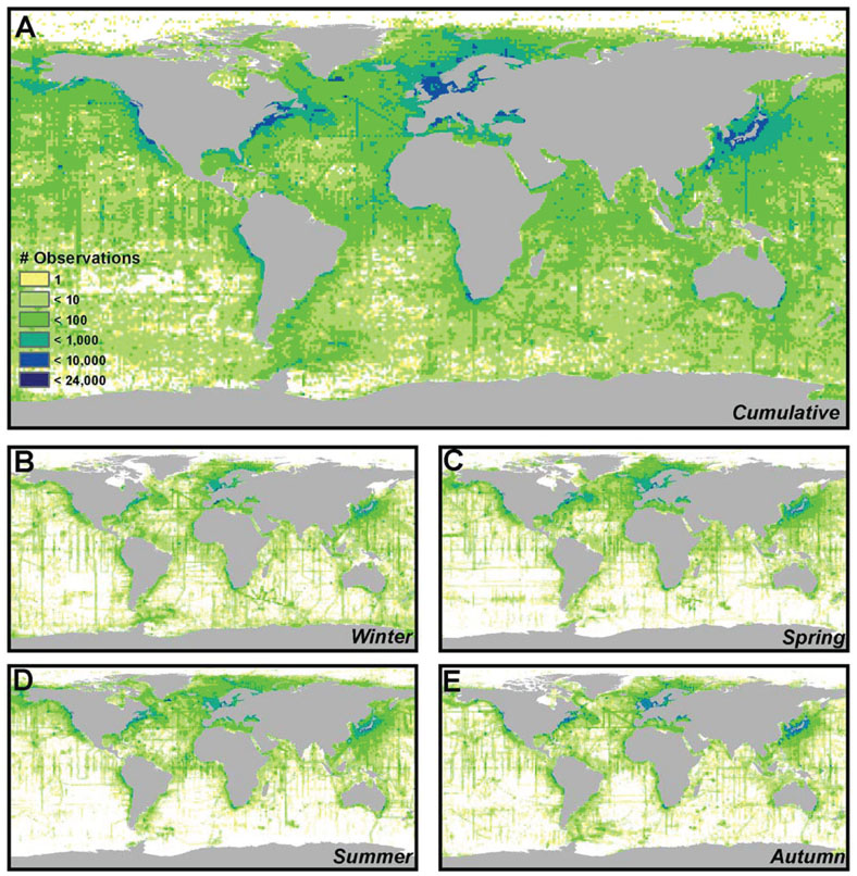
We have represented the error due to spatial/temporal bias in the original salinity WOA09 dataset in Fig. 1. Spatial bias is evident in Fig. 1A, with more observations being seen near shore and in the northern hemisphere than offshore or in the southern hemisphere. Temporal biases are evident as well (Fig. 1B-E), with the fewest data points collected in the Boreal Autumn months (n = 375,973) and the most data points collected in the Boreal Summer months (n = 664,075). The Boreal Spring (n = 560,708) and Boreal Winter (n = 438,305) were intermediate. Interactions between spatial and temporal biases are also evident. For example, more data is collected in the Southern Ocean during the Boreal Winter (Austral Summer) than during other times of year.

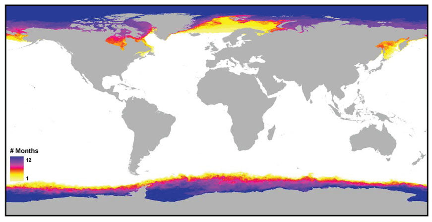
Persistent Ice Cover in SST Data set

We have represented the number of months the sea surface was obscured from the MODIS satellite view by ice coverage in Fig. 2. MARSPEC bioclimatic variables related to temperature were calculated only from ice-free months, and therefore may be biased in regions with permanent or semi-permanent ice coverage. These biases due to ice coverage only affect high latitudes, and we have provided a raster file indicating the number of months each pixel was obscured by ice so that the user can mask out any affected areas for their individual study (see below). Generally speaking, cloud coverage affected much smaller areas and we were able to interpolate the values of pixels missing data due to cloud coverage.

Error Due to Data Smoothing/Interpolation

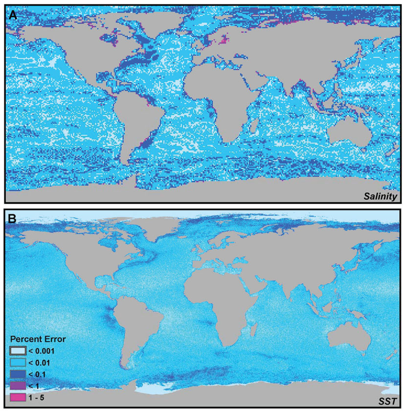
To quantify the error due to spatial interpolation for mean annual sea surface temperature and salinity, we calculated the mean of the high-resolution pixels at 30 arc-seconds contained within neighborhoods equivalent to the native resolution of the original data sets (1 arc-degree for salinity and 2.5 arc-minutes for temperature) using the mean aggregation function in ArcGIS 9.3.1. We then calculated the percent difference between these interpolated/aggregated rasters and the data values of the original data sets. The results are shown in Fig. 3 below.

Overall, salinity exhibited a greater percent difference between original and interpolated data values than temperature, although the error never exceed 5% at any pixel (Fig. 3A). The greatest sources of error in salinity interpolations were observed in areas of transition between ocean masses of differing salinities and around the mouths of major rivers. Furthermore, greater interpolation error was also observed in the polar regions, possibly due to steep transitions between areas of low and high salinity. The areas showing the least amount of interpolation error were those in the open ocean, where oceanographic conditions are stable over greater geographic areas.

Interpolation error for SST was very small, with the percent difference between original and interpolated data values rarely exceeding 0.01%, and never exceeding 0.1% (Fig. 3B). Spatial error seemed to be the greatest at the edges of oceanographic fronts and in areas of seasonal ice cover. Not surprisingly, areas with permanent ice cover (i.e., with values of -2ºC) exhibited no interpolation error.

Implications for the End-User

For the end-user, error in the MARSPEC variables due to data deficiencies should be of greater concern than error introduced by data smoothing/interpolation. Strong spatial and temporal collection biases were observed in both salinity and SST datasets, however the impacts of such biases on the MARSPEC data set differ, and the implications for the end-user will ultimately depend on the area of interest and type of organism under study. The most egregious source of error for polar scientists arises from seasonal ice cover in the SST MODIS images, since estimates of annual mean, range, and variance as well as the temperature of the coldest month are calculated over only the ice-free months of the year. The result is that mean annual SST and temperature of the coldest month are upwardly biased in some polar regions, while range and variance may be underestimated. As applied to ecological niche models, such biases could result in over-prediction of cold-temperate species into polar-regions and may serve as an incorrect baseline for future climate models. Investigators interested in benthic or pelagic species capable of living under the sea-ice during winter months may wish to supplement the MARSPEC dataset with in situ measurements or from an ocean general circulation model such as the HYbrid Coordinate Ocean Model (http://www.hycom.org). Biogeo14 (SST of the coldest ice-free month) may be useful to investigators interested in modeling the ranges of migratory species, such as whales or some seabirds, that are only found in the polar regions during ice-free times of the year. Furthermore, biogeo15 (SST of the warmest ice-free month) may be a useful variable to all end-users since it is measured with no error with respect to ice cover (with the exception of regions covered by permanent sea-ice) and is highly correlated with biogeo14 globally. For investigators wishing to mask out regions affected by seasonal or permanent sea-ice, we have provided a raster layer indicating the number of months the pixel value is obscured by sea-ice as shown in Fig. 2.

Although data deficiencies in the salinity variables are more widely distributed across the globe, they may be of less concern to the end user in most regions of the world. Coastal regions, where salinity gradients are most pronounced, tend to be more data rich than most regions of the open ocean, particularly in the northern hemisphere where sampling is most dense along both coasts of North America, northern Europe, and Japan and is less seasonally biased than the open ocean. Salinity gradients found in these regions will be well characterized by the dataset and can be used in ecological niche models without fear of spatial or temporal bias. Furthermore, data poor regions of the open ocean tend to have the lowest levels of spatial and temporal environmental heterogeneity. As such, low sampling density in regions of the South Pacific, Indian, South Atlantic, and Southern Oceans may be inconsequential since interpolation across broad spatial scales does not typically encompass steep salinity gradients. Users should be most suspect of the salinity data when their region of interest includes sharp salinity gradients in coastal regions of the southern hemisphere, including the mouths of estuaries, along oceanic fronts, and in regions of strong upwelling, since data deficiencies in these regions may result in a misrepresentation of the spatial gradient. Insufficient sampling may fail to capture extreme events such as seasonal upwelling or changes in freshwater efflux in data deficient regions, resulting in an overestimation of cline widths in regions of transition between fresh and saltwater and therefore and overestimation in species ranges in niche models. Furthermore, it is not appropriate to use the MARSPEC database in estuaries in any part of the world. Users interested in studying the distribution of organisms in shallow, data poor regions of the world or in estuarine environments should supplement this dataset with in situ measurements from data loggers or buoys. Ultimately, end-users should inspect Fig. 1 in their region of interest to determine if observational biases in the salinity data set may affect their study.

ADDITIONAL HIGH RESOLUTION RASTER FILES:

A. Data set file

Identity: Sea_Ice_30s.7z

Size: 2,123,440 bytes

Format and storage mode: This layer is provided as an ESRI raster grid at 30 arc-second spatial resolution and compressed into a single 7-zip archive. 7-zip archives can be unpacked with various zip utility programs, including 7-Zip 9.20 (open-source, http://www.7-zip.org/) and WinZip (proprietary, http://www.winzip.com). This ESRI grids is unprojected in the WGS84 Geographic Coordinate System.

Special characters: Land is given as NoData.

B. Variable information:

This ESRI raster grid gives the number of months the measurement of sea surface temperature by satellite was obscured by seasonal or permanent sea ice. It is the source for Fig. 2 above.

C. Data anomalies: N/A

LOWER RESOLUTION MARSPEC DATA FILES:

A.1 Data set file

Identity: MARSPEC_2o5m.7z

Size: 441,194,773 bytes

Format and storage mode: ESRI raster grids at 2.5 arc-minute spatial resolution (approximately 5 km grid cell sizes at the equator) for the temperature and salinity monthly climatologies, bathymetry, and derived geophysical and bioclimatic variables (see Table 1) are compressed together in a single 7-zip archive.7-zip archives can be unpacked with various zip utility programs, including 7-Zip 9.20 (open-source, http://www.7-zip.org/) and WinZip (proprietary, http://www.winzip.com). All ESRI grids are unprojected in the WGS84 Geographic Coordinate System.

Special characters: Land is given as NoData.

A.2 Data set file

Identity: MARSPEC_5m.7z

Size: 128,289,238 bytes

Format and storage mode: ESRI raster grids at 5 arc-minute spatial resolution (approximately 10 km grid cell sizes at the equator) for the temperature and salinity monthly climatologies, bathymetry, and derived geophysical and bioclimatic variables (see Table 1) are compressed together in a single 7-zip archive. 7-zip archives can be unpacked with various zip utility programs, including 7-Zip 9.20 (open-source, http://www.7-zip.org/) and WinZip (proprietary, http://www.winzip.com). All ESRI grids are unprojected in the WGS84 Geographic Coordinate System.

Special characters: Land is given as NoData.

A.3 Data set file

Identity: MARSPEC_10m.7z

Size: 36,738,322 bytes

Format and storage mode: ESRI raster grids at 10 arc-minute spatial resolution (approximately 20 km grid cell sizes at the equator) for the temperature and salinity monthly climatologies, bathymetry, and derived geophysical and bioclimatic variables (see Table 1) are compressed together in a single 7-zip archive. 7-zip archives can be unpacked with various zip utility programs, including 7-Zip 9.20 (open-source, http://www.7-zip.org/) and WinZip (proprietary, http://www.winzip.com). All ESRI grids are unprojected in the WGS84 Geographic Coordinate System.

Special characters: Land is given as NoData.

B. Variable information: As above in Table 1 for high-resolution data files

C. Data anomalies: As above in high-resolution data files.

Class V. Supplemental descriptors

A. Data acquisition

Data forms or acquisition methods: N/A

Location of completed data forms: N/A

Data entry/verification procedures: N/A

B. Quality assurance/quality control procedures: See Class IV.C – Data anomalies section.

C. Related material: N/A

D. Computer programs and data processing algorithms: All data processing was performed in ArcGIS 9.3.1 as described above. Tutorials for clipping the data sets (in ArcGIS and non-proprietary software) to smaller areas of interest and converting to ASCII format, which is required by most ecological niche modeling programs, can be found at the primary author’s website:  http://www.marspec.org.

E. Archiving: N/A

F. Publications and results:

Sbrocco, E. J. 2012. A Seascape Genetics Approach to Exploring the Phylogeographic Response of Marine Fishes to Late Quaternary Climate Change. Boston University. United States -- Massachusetts: ProQuest Dissertations & Theses (PQDT).

Waltari, E., and M. J. Hickerson. 2012. Late Pleistocene species distribution modelling of North Atlantic intertidal invertebrates. Journal of Biogeography. doi: 10.1111/j.1365-2699.2012.02782.x

G. History of data set usage:

The MARSPEC dataset has been disseminated to approximately one dozen scientists interested in modeling the spatial distributions of variety of marine species from around the world. With the exceptions listed above, projects are in the early stages of completion. The MARSPEC dataset was also applied to questions in marine ecological niche modeling and niche divergence in the dissertation of the lead author with further publications are pending as of 1 August 2012.

Acknowledgments

EJS was supported by research and teaching fellowships from Boston University’s Department of Biology and by National Science Foundation grant OCE-0349177 (Biological Oceanography) to PHB during the development of MARSPEC. EJS received support from NSF Coral Triangle PIRE grant OISE-0730256 to PHB and by NSF grant EF-0905606 through the National Evolutionary Synthesis Center (NESCent) during the writing of the manuscript. We thank CJ Schneider and two anonymous reviewers for comments that improved the manuscript.

Literature cited

Antonov, J. I., D. Seidov, T. P. Boyer, R. A. Locarnini, A. V. Mishonov, H. E. Garcia, O. K. Baranova, M. M. Zweng, and D. R. Johnson. 2010. World Ocean Atlas 2009, Volume 2: Salinity. S. Levitus, editor. NOAA Atlas NESDIS 69. U.S. Government Printing Office, Washington, D.C., USA.

Becker, J. J., D. T. Sandwell, W. H. F. Smith, J. Braud, B. Binder, J. Depner, D. Fabre, J. Factor, S. Ingalls, S-H. Kim, R. Ladner, K. Marks, S. Nelson, A. Pharaoh, R. Trimmer, J. Von Rosenberg, G. Wallace, and P. Weatherall. 2009. Global Bathymetry and Elevation Data at 30 Arc Seconds Resolution: SRTM30_PLUS. Marine Geodesy 32:355–371.

Bost, C. A., C. Cotte, F. Bailleul, Y. Cherel, J. B. Charrassin, C. Guinet, D. G. Ainley, and H. Weimerskirch. 2009. The importance of oceanographic fronts to marine birds and mammals of the southern oceans. Journal of Marine Systems 78:363–376.

Briggs, J. C. 1974. Marine Zoogeography. McGraw-Hill< new York, New York, USA.

Briggs, J. C. 1995. Global Biogeography. Elsevier, Amsterdam, The Netherlands.

Cromwell, T., and J. L. Reid. 1956. A study of oceanic fronts. Tellus 8:94–101.

Diniz-Filho, J. A. F., L. C. Terribile, M. J. R. da Cruz, and L. C. G. Vieira. 2010. Hidden patterns of phylogenetic non-stationarity overwhelm comparative analyses of niche conservatism and divergence. Global Ecology and Biogeography 19:916–926.

Elith, J., C. H. Graham, R. P. Anderson, M. Dudik, S. Ferrier, A. Guisan, R. J. Hijmans, F. Huettmann, J. R. Leathwick, A. Lehmann, J. Li, L. G. Lohmann, B. A. Loiselle, G. Manion, C. Moritz, M. Nakamura, Y. Nakazawa, J. M. Overton, A. T. Peterson, S. J. Phillips, K. Richardson, R. Scachetti-Pereira, R. E. Schapire, J. Soberon, S. Williams, M. S. Wisz, and N. E. Zimmermann. 2006. Novel methods improve prediction of species' distributions from occurrence data. Ecography 29:129–151.

Fautin, D. G., and R. W. Buddemeier. 2008. Biogeoinformatics of the Hexacorals: http://www.kgs.ku.edu/Hexacoral/.

Galarza, J. A., J. Carreras-Carbonell, E. Macpherson, M. Pascual, S. Roques, G. F. Turner, and C. Rico. 2009. The influence of oceanographic fronts and early-life-history traits on connectivity among littoral fish species. Proceedings of the National Academy of Sciences of the United States of America 106(5):1473–1478.

Garcia, H. E., R. A. Locarnini, T. P. Boyer, J. I. Antonov, O. K. Baranova, M. M. Zweng, and D. R. Johnson. 2010a. World Ocean Atlas 2009, Volume 3: Dissolved Oxygen, Apparent Oxygen Utilization, and Oxygen Saturation. S. Levitus, editor. NOAA Atlas NESDIS 70. U.S. Government Printing Office, Washington, D.C., USA.

Garcia, H. E., R. A. Locarnini, T. P. Boyer, J. I. Antonov, M. M. Zweng, O. K. Baranova, and D. R. Johnson. 2010b. World Ocean Atlas 2009, Volume 4: Nutrients (phosphate, nitrate, silicate). S. Levitus, editor. NOAA Atlas NESDIS 71. U.S. Government Printing Office, Washington, D.C., USA.

Herborg, L. M., C. L. Jerde, D. M. Lodge, G. M. Ruiz, and H. J. Macisaac. 2007. Predicting invasion risk using measures of introduction effort and environmental niche models. Ecological Applications 17:663–674.

Hijmans, R. J., S. E. Cameron, J. L. Parra, P. G. Jones, and A. Jarvis. 2005. Very high resolution interpolated climate surfaces for global land areas. International Journal of Climatology 25:1965–1978.

Locarnini, R. A., A. V. Mishonov, J. I. Antonov, T. P. Boyer, H. E. Garcia, O. K. Baranova, M. M. Zweng, and D. R. Johnson. 2010. World Ocean Atlas 2009, Volume 1: Temperature. S. Levitus, editor. NOAA Atlas NESDIS 68. U.S. Government Printing Office, Washington, D.C., USA.

Peterson, A. T., M. A. Ortega-Huerta, J. Bartley, V. Sánchez-Cordero, J. Soberón, R. H. Buddemeier, and D. R. B. Stockwell. 2002. Future projections for Mexican faunas under global climate change scenarios. Nature 416:626–629.

Raxworthy, C. J., E. Martinez-Meyer, N. Horning, R. A. Nussbaum, G. E. Schneider, M. A. Ortega-Huerta, and A. T. Peterson. 2003. Predicting distributions of known and unknown reptile species in Madagascar. Nature 426:837–841.

Roberts, J. J., B. D. Best, D. C. Dunn, E. A. Treml, and P. N. Halpin. 2010. Marine Geospatial Ecology Tools: An integrated framework for ecological geoprocessing with ArcGIS, Python, R, MATLAB, and C++. Environmental Modelling & Software 25:1197–1207.

Robinson, L. M., J. Elith, A. J. Hobday, R. G. Pearson, B. E. Kendall, H. P. Possingham, and A. J. Richardson. 2011. Pushing the limits in marine species distribution modelling: lessons from the land present challenges and opportunities. Global Ecology and Biogeography 20:789–802.

Rocha, L. A. 2003. Patterns of distribution and processes of speciation in Brazilian reef fishes. Journal of Biogeography 30:1161–1171.

Seo, C., J. H. Thorne, L. Hannah, and W. Thuiller. 2009. Scale effects in species distribution models: implications for conservation planning under climate change. Biology Letters 5:39–43.

Spalding, M. D., H. E. Fox, G. R. Allen, N. Davidson, Z. A. Ferdaña, M. Finlayson, B. S. Halpern, M. A. Jorge, A. Lombana, S. A. Lourie, K. D. Martin, E. McManus, J. Molnar, C. A. Recchia, and J. Robertson. 2007. Marine ecoregions of the world: A bioregionalization of coastal and shelf areas. BioScience 57:573–583.

Tabor, K., and J. W. Williams. 2010. Globally downscaled climate projections for assessing the conservation impacts of climate change. Ecological Applications 20:554–565.

Tyberghein, L., H. Verbruggen, K. Pauly, C. Troupin, F. Mineur, and O. De Clerck. 2011. Bio-ORACLE: a global environmental dataset for marine species distribution modelling. Global Ecology and Biogeography 21:272–281.

Waltari, E., R. J. Hijmans, A. T. Peterson, A. S. Nyári, S. L. Perkins, and R. P. Guralnick. 2007. Locating pleistocene refugia: Comparing phylogeographic and ecological niche model predictions. PLoS ONE 2:e563.

Wessel, P., and W. H. F. Smith. 1996. A Global Self-consistent, Hierarchical, High-resolution Shoreline Database. Journal of Geophysical Research 101:8741–8743.

Zimmermann, N. E., T. C. Edwards, C. H. Graham, P. B. Pearman, and J. C. Svenning. 2010. New trends in species distribution modelling. Ecography 33:985–989.

Table 1. Definitions of monthly climatologies and derived (core) bioclimatic and geophysical MARSPEC layers. Dividing variable by scaling factor returns the integer value to the unscaled floating point value. SST = sea surface temperature, SSS = sea surface salinity, psu = practical salinity units, WOA09 = World Ocean Atlas 2009.

Fig. 1. Sea Surface Salinity Collection Bias in the WOA09 Dataset.

Fig. 2. The number of months the measurement of sea surface temperature by satellite was obscured by seasonal or permanent sea ice.

Fig. 3. Error introduced by interpolation/data smoothing in (A) salinity and (B) temperature data sets.

[Back to E094-086]