Ecological Archives E094-050-A2

Marion Tafani, Aurelie Cohas, Christophe Bonenfant, Jean-Michel Gaillard, and Dominique Allainé. 2013. Decreasing litter size of marmots over time: a life history response to climate change? Ecology. 94:580–586. http://dx.doi.org/10.1890/12-0833.1

Appendix B. Complementary analyses using seasonal indices.

To analyse temporal variation in litter size of Alpine marmots, we used both single weather variables and seasonal indices to describe previous summer, winter and spring conditions experienced by marmots Although we were able to identify a set of climatic factors critical for litter size variation of Alpine marmots, synthetic indices representing each season (summer and winter preceding reproduction and spring of reproduction) were also considered (Grosbois et al. 2008) to avoid missing important effects (Hallett et al. 2004).

Methods

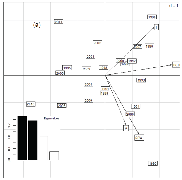
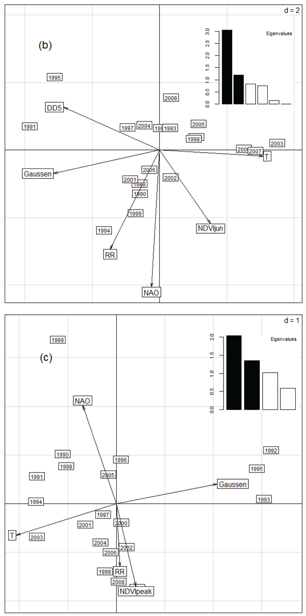
Principal Component Analyses (PCA) were performed to obtain yearly measures of seasonal weather (Stenseth and Mysterud 2005). Daily precipitation, air temperature, and snow depth were all recorded from the weather stations of Tignes and Val d’Isère, 5 km away from the study site. Winter, spring and summer were characterized by the first Principal Component of the respective PCAs (Fig. B1). The winter index encompassed total rainfall, average air temperature, average snow depth, and the North Atlantic Oscillation index (NAO, Hurrell 1995) from December to March (Fig. B1a). For the spring index, the former variables were calculated from April to mid-June in addition to the Bagnoul Gaussen Index (BGI, Bagnouls and Gaussen 1953), the number of days with an average air temperature under 5°C during a month (degree day 5°C) and the Normalized Difference Vegetation Index (NDVI, available up to 2008 from the NOAA, grid size of 8 × 8 km, Tucker et al. 1991) recorded in June, which measures the plant productivity in mid-spring (Pettorelli et al. 2005) were all included in the PCA (Fig. B1b). The summer index included average temperature, precipitation, NAO, BGI from mid-June to August and the date when primary productivity is highest (NDVI peak) (Fig. B1c).

We used linear models to search for temporal trends in climatic variables. When a trend was detected, we used the residuals from the regression between the climatic variable and year as a “de-trended variable”, which can be interpreted as the temporal variation in a climatic variable around the trend, instead of the raw variable to avoid spurious correlations (Grosbois et al. 2008). We fitted Generalized Estimating Equations (GEE) models including female identity as a grouping factor to account for repeated measurements of the same individuals and mother age as a three-level fixed factor (unknown, prime-age, and old) to account for age variation in litter size (Berger et al., in prep). We then modeled litter size variation in relation to time and environmental variables (estimates and SE). In all models including a de-trended variable, year was added to account for the trend (Grosbois et al. 2008). The choice of GEE was motivated by its strong robustness compared to Generalized Linear Mixed Models (GLMM) (Diggle 2002). We then measured the relative effects of each variable in a model using a deviance analysis (ANODEV, Skalski et al. 1993). We used GLMMs to estimate the log-likelihood of each model. ANODEV corresponds to a comparison between the covariate model, and both the constant (i.e., null model) and the time-dependent (i.e., including year as a discrete factor) models. The corresponding F_cst/co/t statistic tests the null hypothesis that the climatic covariate has no effect on litter size; while the r² of the ANODEV quantifies how much of the temporal variation in litter size is accounted for by each climatic model (Grosbois et al. 2008) (see r² dev in Table B1).

Results

Environmental trends

Winter principal components decreased (-0.12±0.03, p < 0.001), while spring principal components increased (0.17±0.07, p = 0.02) over years, thereby documenting a thinner snow layer from December to March and warmer and dryer springs from April to mid-June. The summer principal component decreased over years (-0.15±0.06, p = 0.02), indicating wetter and milder summers in recent years. Overall, climate indices support the recent changes observed in the Alps (Beniston et al. 2003, see main text).

Litter size variation with seasonal indices under climate change

Litter size was positively correlated with winter index (0.050±0.021, p = 0.007, Table B1), meaning that litter size decreased with severe winters characterized by a thinner snow layer and a low air temperature. Nevertheless, the model only including snow cover in winter outperformed the model including winter severity (Table B1). The spring index, mostly driven by temperature and NDVI, had a positive effect on litter size (0.026±0.018, p = 0.04, Table B1) when added to snow cover in winter. However, once again, the model with additive effects of snow cover in December–March and NDVI in April outperformed the model including snow cover in December–March and the spring index (see main text). The summer index did not account for litter size variation over years (-0.019±0.019, p = 0.13, Table B1).

Discussion

A mild winter with warm temperature and deep snow cover from December to March is likely to favor the reproductive output of Alpine marmots. The climatic trend was actually the reverse, and should lead to a decrease in the reproductive output of Alpine marmots with time. Those results support our findings on litter size (see main article). Nevertheless, since at least two axes were necessary to fully capture the seasonal weather variability (Fig. B1), PCAs were not competitive with single variables and were not presented in the main text.

Table B1. Climatic variables accounting for litter size variation of Alpine marmots at La Grande Sassière (Alps, France). “De-trended” variables, entered in the model with their trend stated as “(Year)”, appear in italics. Climatic effects are tested with an analysis of deviance (ANODEV, see methods for details). F statistic of ANODEV (F_cst/co/t) and its associated value (p(F)) test the climatic covariate effect on litter size whiler²dev gives its magnitude. The totalr²of a model with several covariates is written as r²tot. Statistically significant variables are bolded.

*First Principal Component

Fig. B1. Seasonal indices (two first Principal Components). Indices are built upon Principal Component Analyses using local weather variables as loadings. In each panel the x and y axis represent respectively the first and second Principal Components (PC), and arrows represent the relative contribution of climatic covariates to PCs. Eigen values give the relative percentage of total inertia carried by each PC (filled bars are the eigen values of the two PCs displayed on the figure). Individual climatic variables are measured from (a) December to March for the winter index, (b) April to mid-June for the spring index, and (c) mid-June to August the year before for the summer index. T = temperature, RR = precipitations, gaussen = Gaussen index, DD5 = Degree Day 5.

Literature Cited

Bagnouls, F., and H. Gaussen. 1953. Saison sèche et indice xérothermique. Bulletin de la Societé d’Histoire Naturelle de Toulouse 88:193–239.

Beniston, M., F. Keller, B. Koffi, and S. Goyette. 2003. Estimates of snow accumulation and volume in the Swiss Alps under changing climatic conditions. Theoretical and Applied Climatology 76:125–140.

Diggle, P. J. 2002. Analysis of longitudinal data. Oxford University Press, Oxford, UK.

Grosbois, V., O. Gimenez, J. M. Gaillard, R. Pradel, C. Barbraud, J. Clobert, A. P. Møller, and H. Weimerskirch. 2008. Assessing the impact of climate variation on survival in vertebrate populations. Biological Reviews 83:357–399.

Hallett, T. B., T. Coulson, J. G. Pilkington, J. M. Pemberton, and B. T. Grenfell. 2004. Why large-scale climate indices seem to predict ecological processes better than local weather. Nature 430:71–75.

Hurrell, J. W. 1995. Decadal trends in the North-Atlantic Oscillation - Regional temperatures and precipitations. Science 269:676–679.

Pettorelli, N., J. O. Vik, A. Mysterud, J.-michel M. Gaillard, C. J. Tucker, N. C. Stenseth, and C. B. Lyon. 2005. Using the satellite-derived NDVI to assess ecological responses to environmental change. Trends in Ecology and Evolution 20:503–10.

Skalski, J. R., A. Hoffman, and S. G. Smith. 1993. Testing the significance of individual- and cohort-level covariates in animal survival studies. Pages 9–28 in J. D. Lebreton and P. M. North, editors. Marked individuals in the study of bird population. Birkaüser Verlag, Basel, Switzerland.

Stenseth, N. C., and A. Mysterud. 2005. Weather packages : finding the right scale and composition of climate in ecology. Journal of Animal Ecology 74:1195–1198.

Tucker, C. J., W. W. Newcomb, S. O. Los, and S. D. Prince. 1991. Mean and inter-year variation of growing-season Normalized Difference Vegetation Index for the Sahel 1981-1989. International Journal of Remote Sensing 12:1133–1135.

[Back to E094-050]