Daniel J. McGlinn, Peter G. Earls, and Michael W. Palmer. 2010. A 12-year study on the scaling of vascular plant composition in an Oklahoma tallgrass prairie. Ecology 91:1872.

Abstract: We present data that were collected as part of a monitoring project on vascular plant composition at the Tallgrass Prairie Preserve in Osage County, Oklahoma, USA. The purpose of these data are to promote the study of multi-scale patterns of species composition for both theoretical and applied questions. Furthermore, these data will provide a reference point for tallgrass prairie restoration projects in the Flint Hills. Over the course of the 12-year period, we sampled 20 permanent plots annually. The permanent plots were selected semi-randomly from a UTM grid using the criteria that they contain less than 20% of woody cover, standing water, or exposed rock. Plant species presence was recorded at five spatial scales: 0.01, 0.1, 1.0, 10, and 100 m² in each of the four corners of a 100-m² square quadrat. Plant species were assigned to a percent cover class at the 100-m² grain. In addition to information on plant composition, we provide data on topography, soil variables, monthly total rainfall, monthly average temperature, and management records related to fire and grazing history. We hope this data set will stimulate further research into the scaling of biodiversity and insight into the functioning and conservation of tallgrass prairie plant communities.

Key words: bison; Flint Hills; restoration; spatial scale; species-time-area relationship; tallgrass prairie; vascular plants; vegetation monitoring.

INTRODUCTION

Patterns of species richness are scale dependent. This simple fact has provided clues into the drivers of richness and challenged our understanding of biodiversity. For example, the well known species-area relationship is an expression of how species richness changes as a function of spatial grain. This relationship has revealed how a diverse array of factors influence the scale dependence of species richness, including the rarefaction effect (McGlinn and Palmer 2009), environmental heterogeneity (Palmer 2007a), dispersal limitation (Rosenzweig 1995), and evolutionary isolation (Drakare et al. 2006). Indeed, it is now relatively common place for ecologists to consider patterns of richness at multiple spatial scales. However, time, another important facet of scale, has received considerably less attention in studies of biodiversity (White et al. 2006a, White 2007). This omission occurred despite early recognition that the temporal scale of a sample is an important determinate of richness (Fisher et al. 1943, Preston 1960). The importance of considering the temporal scaling of diversity is compounded by the growing body of evidence that demonstrates that the scaling of richness in space depends upon the temporal scale over which it is examined (Adler et al. 2005, Fridley et al. 2005, McGlinn and Palmer 2009). The interdependence of the spatial and temporal scaling of diversity (i.e., the species-time-area relationship, STAR) has the potential to provide new theoretical insights by requiring that models simultaneously account for changes in diversity in space and time (e.g., Adler 2004).

Applied ecology also may benefit through the development of novel methods for carrying out space-for-time substitutions (Adler and Lauenroth 2003, Adler et al. 2005). One potential application of space-for-time substitutions is to predict future temporal patterns of diversity in light of climate change with the aid of current spatial patterns of diversity (Adler and Levine 2007).

Given the importance of temporal patterns of diversity, it appears that the current paucity of studies on temporal scaling of diversity is due in large part to a lack of suitable data sets in the public domain. Here, we describe a multi-scale data set in space and time on vascular plants that can be utilized to address questions related to the scaling of species richness in space and time. Portions of this data set have already addressed a range of applied and theoretical questions. Palmer et al. (2002) used part of this data set to compare strategies for efficiently conducting a thorough taxonomic inventory. Palmer et al. (2003) examined the relevance of the species pool hypothesis to explain the relationship between species richness and soil reaction. Brokaw (2004) compared the ability of modern measures of the soil environment (e.g., total C, residual P) with traditional measures of soil properties (e.g., soil cations) to explain plant composition using only samples in this data set collected in 2002. Palmer et al. (2008) examined how the relationships between native and exotic richness as well as the species to genus ratio changed as a function of scale. McGlinn and Palmer (2009) constructed an empirical example of a STAR with the data. M.W. Palmer has also used the data to provide The Nature Conservancy progress reports related to changes in the vegetation of the Tallgrass Prairie Preserve (TGPP).

In addition to stimulating additional studies into the relationship of biodiversity and scale, this data set will be valuable to practitioners interested in the dynamics and conservation of the tallgrass prairie ecosystem.

METADATA

CLASS I. DATA SET DESCRIPTORS

A. Data set identity:

Title: Multi-scale vascular plant composition from long-term monitoring at the Tallgrass Prairie Preserve, Oklahoma

B. Data set identification code:

Suggested Data Set Identity Code: TGPP_plants

C. Data set description

Principal Investigator: Michael W. Palmer, Department of Botany, Oklahoma State University, Oklahoma, USA.

Daniel J. McGlinn, Department of Botany, Oklahoma State University, Oklahoma, USA (Department of Biology, University of North Carolina, Chapel Hill, North Carolina, USA).

Abstract: as above

D. Key words: as above

CLASS II. RESEARCH ORIGIN DESCRIPTORS

A. Overall project description

Identity: Multi-scale vascular plant composition from long-term monitoring at the Tallgrass Prairie Preserve, Oklahoma

Originator: M. W. Palmer

Period of Study: Multiscale vascular plant data and environmental site data from the month of June, 1998–2009. Climate data from January 1993 to June 2009.

Objectives: To evaluate the species–time–area relationship as well as monitor changes in vegetation in response to the environment.

Abstract: same as above.

Sources of funding: The Oklahoma State University College of Arts and Science, The Oklahoma Nature Conservancy, The Spatial and Environmental Information Clearinghouse, The Philecology Trust, The Swiss Federal Institute for Forest, Snow and Landscape Research, and the Oklahoma Water Resources Research Institute provided financial assistance at various stages of research at the Tallgrass Prairie Preserve.

B. Specific subproject description

Study Site:

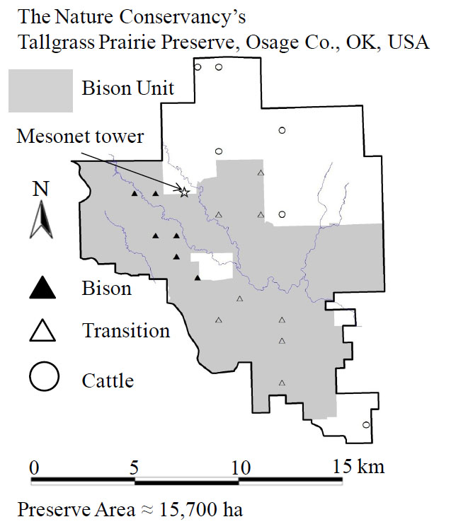
The Tallgrass Prairie Preserve (TGPP, ca. 15,700 ha in size) is located between 36.73° and 36.90° N latitude, and 96.32° and 96.49° W longitude in Osage County, Oklahoma, USA. The elevation on the preserve varies from 253 to 366 m, and over the course of the study period (1998 to 2009) the total annual rainfall averaged 940 mm and ranged from 594 to 1218 mm. The preserve is located in the southern terminus of the Flint Hills (see Hamilton 2007 Fig.1) which is an ecoregion characterized by shallow soils derived from Permian sediment (Oviatt 1998). Due to long-term erosion, the surface layers of the soil are thin and young; limestone and sandstone are frequently exposed at the surface. Because of these shallow rocky soils, the Flint Hills, including the TGPP, has remained unplowed and is utilized primary for cattle grazing (Kindscher and Scott 1997).

The TGPP is owned and operated by The Nature Conservancy (TNC) who purchased the bulk of the preserve (the 11,800 ha Barnard Ranch) in 1989. Since that time the TNC has made additional land acquisitions that increased the preserve’s area to its current size. Prior to the acquisition of the preserve by TNC in 1989, the majority of the site was managed for cow-calf and yearling cattle production with a 4- to 5-year rotation of prescribed burning and aerial application of broadleaf herbicides (1950–1989) (Hamilton 2007). In 1993, 300 bison (Bos bison) were introduced onto a 1,960 ha portion of the preserve. Over time the bison unit has ground grown to a herd size of ca. 2,600 and occupies an area of ca. 8,500 ha (shaded region, Fig. 1). Approximately one-third of the burn units (watersheds) within the bison unit are randomly selected for prescribed burning annually. Some areas experience periods as long as 10 years without fire due to the random nature of burn unit selection. The remainder of the preserve is managed for seasonal cow-calf production with a more frequent application of fire. Lastly, bison are allowed to graze year round, but cattle grazing is only during the spring and summer months. Hamilton (2007) provides additional details on the management of the TGPP.

Approximately 90 % of the TGPP consists of grasslands. The majority of the grasslands are composed of tallgrass prairie habitats dominated by Andropogon gerardii, Sorghastrum nutans, Sporobolus compositus, Panicum virgatum, and Schizachyrium scoparium. Shortgrass prairie habitat occurs to a lesser extent on more xeric sites and is dominated by Bouteloua spp. Other notable vegetation types on the preserve are oak woodlands of the cross timbers which are composed primarily of Quercus stellata and Quercus marilandica, gallery forests along the main tributaries, and ephemeral wetland communities on shallow slopes and plateaus. Despite the application of herbicide earlier in the 20th century, the flora of the TGPP appears relatively intact with a total of 763 species of vascular plants present (to date) of which 12.1% are exotic (Palmer 2007b). The referenced voucher specimens for our study are deposited in two locations: 1) in the Oklahoma State University Herbarium (herbarium code: OKLA), Stillwater, OK 74074 and 2) in the TGPP Herbarium, Pawhuska, OK (located at the study site).

Research methods:

A suitable sampling design for understanding the scaling of diversity within and amongst samples requires objectively placed permanent plots. This is necessary to ensure that the results are not biased by the investigators’ subjective impression of homogeneity or representativeness of the site (Palmer 1993). Other important aspects of suitable long-term data include accurately relocating the samples and maintaining the consistency and accuracy of taxa identification (Milberg et al. 2008). Therefore we selected twenty permanent 100 m² plots randomly from a UTM NAD27 1 × 1 km grid of 151 plots. The only criteria we imposed on plot selection were that plots not contain artificial structures or more than 20% of woody cover, standing water, or exposed rock.

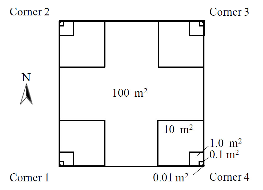
We sampled the plots every June (when we could readily identify both early and late-season plants) from 1998 to 2009. Depending on weather, sampling typically required 10 days in the field to complete. Each plot was 10 × 10 m with iron reinforcement bars at the corners sunk to ground level and topped by Surv-Kap® aluminum caps stamped with the plot ID number. The plots were relocated with a GPS receiver and a magnetic locator. Each corner has a series of square nested subplots with areas of 0.01, 0.1, 1, and 10 m² (Fig. 2). For each subplot (i.e., corner), we recorded the finest grain all vascular plant species were rooted at. If a species was rooted within the plot but not within a subplot then it was not associated with a particular subplot and it was assigned an area of 100 m². We recorded a cover class for each species at the 100 m² grain (Table 2). Species not rooted in the quadrat but leaning into the quadrat were also given a cover class at the 100 m² grain. M. W. Palmer estimated visual cover and made the final identification on all recorded taxa to maintain consistency and accuracy throughout the study. Additionally, we recorded height of the tallest grass, forb, and woody plant; estimated cover of woody plants, rock, bare soil, and water; and recorded slope and aspect. We took two 15 cm deep soil cores 50 cm outside each quadrat corner, for a total of 8 cores per quadrat; we systematically varied the orientation of the soil samples annually to minimize disturbance. Soils were analyzed by Brookside Labs (New Knoxville, OH) for total exchange capacity, pH, percent organic matter, bulk density, and, using a Mehlich 3 extractant, available sulfur, phosphorus, calcium, magnesium, potassium, sodium, boron, iron, manganese, copper, zinc, and aluminum (Mehlich 1984).

Climate data was downloaded from the Foraker Mesonet tower (36.841° N, -96.428° W; elevation: 330 m) that is located on the preserve (Fig. 1). The Mesonet tower is 10 m tall and collects data every 5 minutes on a wide range of meteorologically relevant information (http://www.mesonet.org/mcdguide.pdf; McPherson et al. 2007). However, for the purposes of this data set we only accessed monthly data on total precipitation and average temperature. Precipitation was measured with a Met One Tipping-Bucket Rain Gauge located just off the ground. Temperature was recorded with a Thermometrics Fast Air Temperature sensor 1.5 m above the ground. Although we provide the monthly precipitation and temperature data here, all other measured variables are freely accessible via the Mesonet webpage on a daily interval (http://www.mesonet.org/).

Data on fire events that occurred at the twenty quadrats were extracted from topographic burn maps created by R. G. Hamilton. The burn boundaries were visually digitized in ArcView v3.3 with the aid of a digital 3 m² resolution aerial photograph of the preserve and scanned USGS topographic quadrangle maps. The burn boundaries typically followed the edge of an unpaved road or tributary and are therefore accurate within a reasonable margin of error. Grazing history was reported by R. G. Hamilton and for this data set consists simply of years of bison grazing. All other sites were within cattle units.

The following published works were used as identification guides in the field (Waterfall 1969, McGregor and Barkley 1986, Diggs et al. 1999). Nomenclature follows the PLANTS database (USDA NRCS 2009).

Project personnel:

M. W. Palmer was responsible for establishing the plots, gathering of all species data, data input and error checking. D. J. McGlinn assisted in vegetation sampling, data management, digitizing of burn layers, data input and error checking, and maintenance of the species and environmental components of the data set. P. G. Earls developed the GIS database of management information, assisted in sampling, data input and checking. Many others assisted in the process of sampling the vegetation and soils (see Acknowledgements).

CLASS III. DATA SET STATUS AND ACCESSIBILITY

A. Status

Latest update: January 2010 for the final format of all files.

Latest Archive date: June 2009

Metadata status: Metadata are complete for this period and are stored with the data (see B. below).

Data verification: M. W. Palmer verified all species data. The soil data was checked for consistent values between years by D. J. McGlinn. The management data was extracted by P. G. Earls and D. J. McGlinn.

B. Accessibility

Storage location and medium: All digital data exist on a computer maintained in M. W. Palmer’s laboratory in ASCII format. A backup copy exists on D. J. McGlinn’s computer as well.

Contact person: Michael W. Palmer, Department of Botany, Oklahoma State University, Stillwater Oklahoma 74078 USA; tel 405-744-7717; fax 405-744-7074; [email protected].

Copyright restrictions: None.

Proprietary restrictions: None.

Costs: None.

CLASS IV. DATA STRUCTURAL DESCRIPTORS

A. Data Set File

Identity:

TGPP_pres.csv -- for the species occurrences from 1998 to 2009.

TGPP_cover.csv -- for the species cover classes from 1998 to 2009.

TGPP_rich.csv -- contains species richness for each corner and each level (spatial scale) of each sample.

TGPP_specodes.csv -- for the species names.

TGPP_env.csv -- contains all environmental variables including management and climate information for the study period.

TGPP_clim.csv -- contains monthly total rainfall and average temperature for all years of available Mesnet data, including years prior to the origination of sampling (1994–1997).

Size:

TGPP_pres.csv -- 44508 lines, not including header row.

TGPP_cover.csv -- 18379 lines, not including header row.

TGPP_rich.csv -- 4080 lines, not including header row.

TGPP_specodes.csv -- 320 lines, not including header row.

TGPP_env.csv -- 240 lines, not including header row.

TGPP_clim.csv -- 186 lines, not including header row.

Comments:

TGPP_pres.csv --

For each corner, species occurrence was recorded at the finest grain (smallest scale, Table 1) the species was rooted at. Because the subplots are nested within one another at the corners (Fig. 2), species that occur at a given scale occur in all coarser scales for that corner. For example, if a species is recorded at 1 m² in corner 1, then it is also considered present at 10 m² in corner 1 and at 100 m², the area of the entire plot. If a species was only observed at the 100 m² scale (i.e., it was not present in a subplot but was rooted within the plot), then the corner was designated as NA.

We occasionally observed evidence of spot applications of herbicide to the invasive species Lespedeza cuneata (sericea lespedeza) in the plots. Therefore, trends in this species should be interpreted with respect to this fact. However, this species was never important in any of our plots.

TGPP_cover.csv --

The cover class for each species rooted within or overlapping the plot was recorded in TGPP_cover.csv. The cover classes only apply at the coarsest scale, 100 m². Species overlapping the plot but not rooted within the quadrat were also included in this file. These overlapping species were designated by the data field, ‘rooted_in’.

TGPP_rich.csv --

This is the summed number of species occurring at each scale in each plot in each corner. Only species that were rooted in the plot (i.e., not simply overlapping) were included in the estimate or species richness. Both determined and undetermined taxa were included in the richness estimate.

TGPP_env.csv and TGPP_clim.csv --

The total monthly precipitation and monthly average temperature information in TGPP_env.csv reflects the monthly conditions from June of the previous calendar year to May of the current sampling year. Additionally we provide the data file TGPP_clim.csv, which contains the identical climate data as TGPP_env.csv, as well as, monthly precipitation and temperature records from the four years before the beginning of the study (1994–1998). Therefore the climate data in the two files are redundant in part. We included this redundant information primarily because we felt that others would find it convenient that the climate variables were already included with the other site variables and because we wanted to provide others the option to calculate climatic lag effects for years prior to the beginning of sampling.

Lastly, in the month of February 1998, the rain gauge at the Mesonet tower did not record any data and therefore we provide no estimate of total rainfall for this month.

Format and storage mode: ASCII text, comma delimited. No compression schemes used.

Authentication procedures: For the TGPP_pres.csv data, the sum of the area values for the entire data set is 347,004.2. The spcode is tridflav for row 1000. For TGPP_cover.csv, the sum of the cover column is 39,766. For TGPP_rich.csv, the sum of all the richness values is 99,484. For the TGPP_specodes.csv data, the sum of the spnum column is 51,360. Species #102 is Desmodium marilandicum, and its code is desmmari. For TGPP_clim.csv, the sum of the rain column is 14,714 mm and the sum of the temperature column is 2,672.4. In the sixth month of 1998, the rainfall total is 49 mm and the average temperature was 24.8 °C. In TGPP_env.csv, the sum of total exchange capacity is 4,541.83. In column 15, row 5, the slope is 4.

B. Variable information

TGPP_pres.csv

TGPP_cover.csv

TGPP_rich.csv

TGPP_specodes.csv

TGPP_env.csv

TGPP_clim.csv

CLASS V. SUPPLEMENTAL DESCRIPTORS

A. Data acquisition

Data forms: data forms.

Location of completed data forms: The completed species data forms are stored at Oklahoma State University Department of Botany (M. W. Palmer’s Office). A copy has also been stored inside the herbarium cabinet at the TGPP research station.

B. Quality assurance/quality control procedures: Field sheets were proofed for concerns after every day in the field as well as during digitization.

C. Related material: NA.

D. Computer programs and data processing algorithms: NA.

E. Archiving: NA.

F. Publications and results:

These data have been used in the following publications:

Brokaw, J. M. 2004. Comparing explanatory variables in the analysis of species composition of a tallgrass prairie. Proceedings of the Oklahoma Academy of Science 84:33–40.

McGlinn, D. J., and M. W. Palmer. 2009. Modeling the sampling effect in the species-time-area relationship. Ecology 90:836–846.

Palmer, M. W., J. R. Arévalo, M. C. Cobo, and P. G. Earls. 2003. Species richness and soil reaction in a northeastern Oklahoma landscape. Folia Geobotanica 38:381–389.

Palmer, M. W., P. G. Earls, B. W. Hoagland, P. S. White, and T. Wohlgemuth. 2002. Quantitative tools for perfecting species lists. Environmetrics 13:121–137.

Palmer, M. W., D. J. McGlinn, and J. F. Fridley. 2008. Artifacts and artifictions in biodiversity research. Folia Geobotanica 43:245–257.

G. History of data set usage:see F. above for references that use the data.

H. Data set update history: All of the data were last updated in June 2009.

Review history: NA.

Questions and comments from secondary users: NA.

ACKNOWLEDGMENTS

DJM received funding from the U.S. Environmental Protection Agency (EPA) under the Greater Research Opportunities (GRO) Graduate Program. The U.S. EPA has not officially endorsed this publication, and the views expressed herein may not reflect the views of the Agency. Additionally we thank Bob Hamilton, members of the Laboratory for Innovative Biodiversity Research and Analysis, and the members of the Osage Nation for assistance with field work and continued encouragement of research conducted on the Osage Reservation. J. A. Steets and R. J. Tyrl provided helpful comments that improved this manuscript.

LITERATURE CITED

Adler, P. B. 2004. Neutral models fail to reproduce observed species-area and species-time relationships in Kansas grasslands. Ecology 85:1265–1272.

Adler, P. B., and W. K. Lauenroth. 2003. The power of time: spatiotemporal scaling of species diversity. Ecology Letters 6:749–756.

Adler, P. B., and J. M. Levine. 2007. Contrasting relationships between precipitation and species richness in space and time. Oikos 116:221–232.

Adler, P. B., E. P. White, W. K. Lauenroth, D. M. Kaufman, A. Rassweiler, and J. A. Rusak. 2005. Evidence for a general species-time-area relationship. Ecology 86:2032–2039.

Brokaw, J. M. 2004. Comparing explanatory variables in the analysis of species composition of a tallgrass prairie. Proceedings of the Oklahoma Academy of Science 84:33–40.

Diggs, G. M., B. L. Lipscomb, and R. J. O'Kennon. 1999. Shinners' and Mahler's illustrated flora of North Central Texas. Botanical Research Institute of Texas, Fort Worth, Texas, USA.

Drakare, S., J. J. Lennon, and H. Hillebrand. 2006. The imprint of the geographical, evolutionary and ecological context on species-area relationships. Ecology Letters 9:215–227.

Fisher, R. A., A. Corbet, and C. B. Williams. 1943. The relation between the number of species and the number of individuals in a random sample of an animal population. Journal of Animal Ecology 12:42–58.

Fridley, J. D., R. K. Peet, T. R. Wentworth, and P. S. White. 2005. Connecting fine- and broad-scale species-area relationships of Southeastern US Flora. Ecology 86:1172–1177.

Hamilton, R. G. 2007. Restoring heterogeneity on the Tallgrass Prairie Preserve: applying the fire-grazing interaction model. Pages 163–169 in R. E. Masters and K. E. M. Galley, editors. Proceedings of the 23rd Tall Timbers Fire Ecology Conference: Fire in Grassland and Shrubland Ecosystems. Allen Press, Tall Timbers Research Station, Tallahassee, Florida, USA.

Kindscher, K., and N. Scott. 1997. Land ownership and tenure of the largest land parcels in the Flint Hills of Kansas, USA. Natural Areas Journal 17:131–135.

McGlinn, D. J., and M. W. Palmer. 2009. Modeling the sampling effect in the species-time-area relationship. Ecology 90:836–846.

McGregor, R. L., and T. M. Barkley. 1986. Flora of the Great Plains. University Press of Kansas, Lawrence, Kansas, USA.

McPherson, R. A., C. A. Fiebrich, K. C. Crawford, J. R. Kilby, D. L. Grimsley, J. E. Martinez, J. B. Basara, B. G. Illston, D. A. Morris, K. A. Kloesel, A. D. Melvin, H. Shrivastava, J. M. Wolfinbarger, J. P. Bostic, D. B. Demko, R. L. Elliott, S. J. Stadler, J. D. Carlson, and A. J. Sutherland. 2007. Statewide Monitoring of the Mesoscale Environment: A Technical Update on the Oklahoma Mesonet. Journal of Atmospheric and Oceanic Technology 24:301–321.

Mehlich, A. 1984. Mehlich 3 soil test extraction modification of Mehlich 2 extractant. Communications in Soil Science and Plant Analysis 15:1409–1416.

Milberg, P., J. Bergstedt, J. Fridman, G. Odell, and L. Westerberg. 2008. Observer bias and random variation in vegetation monitoring data. Journal of Vegetation Science 19:633–644.

Oviatt, C. G. 1998. Geomorphology of Konza Prairie. Pages 35–47 in A. Knapp, J. Briggs, D. Hartnett and S. Collins, editors. Grassland Dynamics: Long-term ecological research in tallgrass prairie.  Oxford University Press, New York, New York, USA.

Palmer, M. W. 1993. Potential biases in site and species selection for ecological monitoring. Environmental Monitoring and Assessment 26:277–282.

Palmer, M. W. 2007a. Species-area curves and the geometry of nature. Pages 15–31 in Scaling Biodiversity, Eds. D. Storch, P. L. Marquet, and J. H. Brown. Cambridge University Press, Cambridge, UK.

Palmer, M. W. 2007b. The vascular flora of the Tallgrass Prairie Preserve, Osage county, Oklahoma. Castanea 72:235–246.

Palmer, M. W., J. R. Arévalo, M. C. Cobo, and P. G. Earls. 2003. Species richness and soil reaction in a northeastern Oklahoma landscape. Folia Geobotanica 38:381–389.

Palmer, M. W., P. G. Earls, B. W. Hoagland, P. S. White, and T. Wohlgemuth. 2002. Quantitative tools for perfecting species lists. Environmetrics 13:121–137.

Palmer, M. W., D. J. McGlinn, and J. F. Fridley. 2008. Artifacts and artifictions in biodiversity research. Folia Geobotanica 43:245–257.

Preston, F. W. 1960. Time and space and the variation of species. Ecology 41:611–627.

Rosenzweig, M. L. 1995. Species Diversity in Space and Time. Cambridge University Press, Cambridge, UK.

USDA NRCS. 2008. The PLANTS Database. National Plant Data Center, Baton Rouge, LA 70874-4490 USA.

Waterfall, U. T. 1969. Keys to the Flora of Oklahoma. Published by the author, Oklahoma State University, Stillwater, Oklahoma, USA.

White, E. P. 2007. Spatiotemporal scaling of species richness: patterns, processes, and implications. Pages 325–346 in D. Storch, P. A. Marquet, and J. H. Brown, editors. Scaling Biodiversity. Cambridge University Press, Cambridge, UK.

White, E. P., P. B. Adler, W. K. Lauenroth, R. A. Gill, D. Greenberg, D. M. Kaufman, A. Rassweiler, J. A. Rusak, M. D. Smith, J. R. Steinbeck, R. B. Waide, and J. Yao. 2006. A comparison of the species-time relationship across ecosystems and taxonomic groups. Oikos 112:185–195.

TABLE 1. The linear dimension and area of the five spatial grains are noted below. The area (i.e., the grain) at which a species was first encountered is denoted in TGPP_pres.csv.

TABLE 2. Each species was placed in a visual cover class at the 100-m² grain.  The cover of each species is denoted in TGPP_cover.csv. 

FIG. 1. A map of the Tallgrass Prairie Preserve. The shaded area denotes the bison unit, which increased in area during the study. The Mesonet tower where the climate data was recorded is marked on the map as a star (). The twenty quadrats sampled each year of this study are displayed on the map (as triangles and circles). The sites that were grazed by bison at the beginning of the study (1998) are displayed with filled triangles (), those that transitioned during the study from cattle to bison are denoted by unfilled triangles (), and the other cattle grazed samples are denoted by unfilled circles ().

FIG. 2. Sampling design for the permanent plots. The presence of each species was recorded in each corner at each spatial grain and percent cover was visually estimated at the 100-m2 grain.