Appendix C. Graphics displaying the predictions of the sampling model for five relative abundance distributions (RADs) with different levels of evenness and five values of the replacement rate (R).
All of these figures were created with model parameters equal to those in the main text. Both area and time were varied from 1 to 16384 by successive doublings of scale and the size of the species pool (SP) was 800. Figures C2 through C4 were generated with the aid of the R package dichromat v1.2-2 (Lumley 2008).
|
|
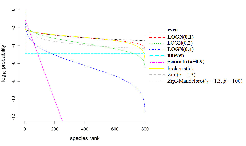
| FIG. C1. The log10 probability rank diagrams for all nine of the different relative abundance distributions (RADs): even, three lognormal, uneven, geometric, broken stick, Zipf, and Zipf-Mandelbrot. Note that the RADs that are bold in the figure legend are the five RADs which were chosen to represent the diversity of possible species-time-area relationships in the manuscript. Also note that the geometric RAD is linear in semi-log space over its entire range and is not shown in its entirety. The least common species in the geometric RAD had a log10 probability of -37.56. |
|
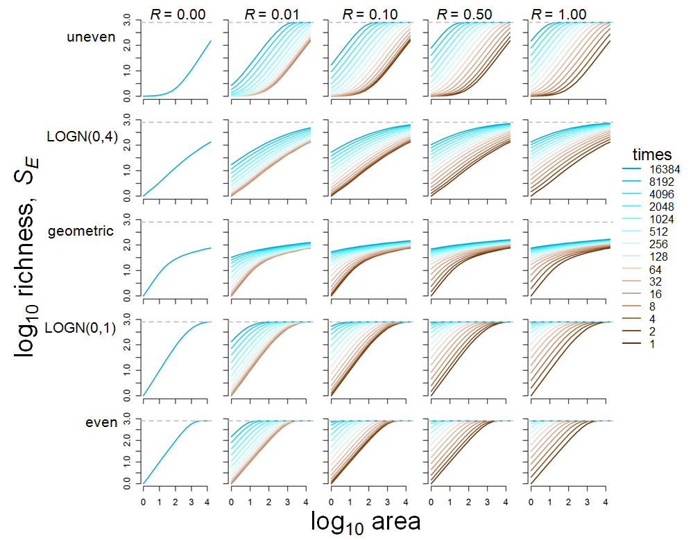
| FIG. C2. The species–area relationship (SAR) for five values of R (columns) and the five RADs (rows). The color of the curves indicate the temporal scale of the SAR (see legend): brown indicates T was small and blue indicates T was large. The dashed grey line indicated the log10 of the size of the species pool, SP. |
|
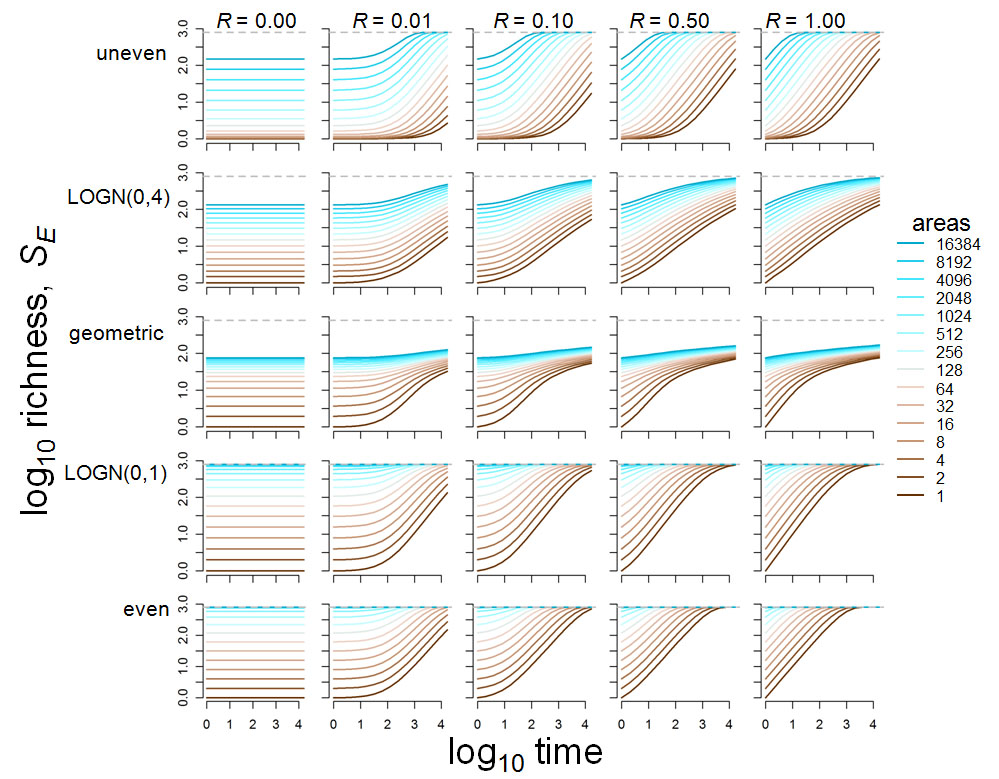
| FIG. C3. The species–time relationship (STR) for five values of R (columns) and the five RADs (rows). The color of the curves indicate the spatial scale of the STR (see legend): brown indicates A was small and blue indicates A was large. The dashed grey vertical line indicated the log10 of the size of the species pool, SP. |
|
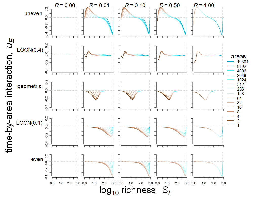
| FIG. C4. The distribution of time-by-area interaction (uE) as a function of log10 richness (SE) for five values of R (columns) and the five RADs (rows). Each curve was generated by holding area constant and varying time. There are no visible curves when R = 0 because uE was equal to zero. Positive values were only observed at fine scales under low evenness. The color of the curves indicate at what scale ur was calculated at (see legend): brown indicates A was small and blue indicates A was large. The dashed horizontal line indicates zero, and the dashed vertical line indicates the log10 size of the species pool, SP. |
LITERATURE CITED
Lumley, T. 2008. Dichromat: color schemes for dichromats. R package version 1.2-2. http://cran.r-project.org/.