Jeremy W. Fox. 2006. Using the Price equation to partition the effects of biodiversity loss on ecosystem function. Ecology 87:2687–2696.

Appendix B. Applications of the Price equation partition to the empirical studies of Wardle et al. (1997), Belnap et al. (2005), and Spehn et al. (2005; the BIODEPTH experiment), and to the theoretical model of Ives and Cardinale (2004).

Here I discuss insights gained from applying the Price Equation partition to the studies of Wardle et al. (1997), Belnap et al. (2005), and Spehn et al. (2005; the BIODEPTH experiment). I also describe the application of the Price Equation partition to the model of Ives and Cardinale (2004).

Analysis of Wardle et al. (1997)

Wardle et al. (1997) measured plant species biomasses on 50 islands in two adjacent Swedish lakes in 1995. The islands vary in area, fire history, plant species richness and composition, and in a variety of other physical and biological variables (e.g., humus mass, soil N content, soil pH). Total plant biomass is the ecosystem function of interest. Species’ biomasses are not available for all of the rare plants, and so for purposes of analysis the 18 most species-rich islands were considered to have 7 species: three tree species and three dwarf shrub species, with the remaining species (which never comprised >3% of total plant biomass) considered as a single species. I compared each less-diverse (“post-loss”) island to each of the most-diverse (“pre-loss”) islands. This procedure provides 18 estimates of the SRE, SCE, and CDE for each of the 32 less-diverse islands.

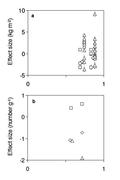
On average less-diverse islands support lower total plant biomass than more-diverse islands, although there is substantial variability around this trend (Fig. B1a). Both positive and negative SCEs and CDEs are observed, although most SCEs are negative (indicating non-random loss of high-biomass species) and most CDEs are positive (indicating increased “post-loss” biomass of the remaining species). To better understand the underlying factors that might drive species loss and context dependence, I conducted multiple regressions of SRE, SCE, and CDE on the difference between pre- and post-loss islands in humus mass, soil N, soil pH, and island size (the latter is a surrogate for many variables; Wardle et al. 1997). I did not include difference in time since most recent fire, since fire history data are unavailable for many post-loss islands. The multiple regressions used mean values of the SRE, SCE, CDE, and predictor variables for each post-loss island, to avoid the non-independence that would arise from using every pairwise comparison between pre-loss and post-loss islands (therefore n = 32 for all regressions). The regression results should be treated cautiously, since the predictor variables are intercorrelated and are not measured without error, but are useful for suggesting hypotheses about the determinants of the SRE, SCE, and CDE.

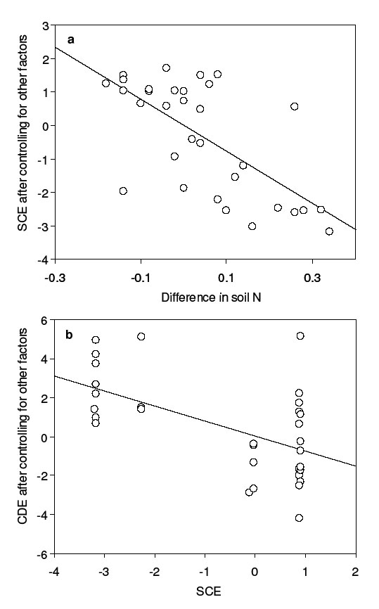
The multiple regression for the SCE is highly significant (R² = 0.53, P < 0.001). The significant multiple regression is attributable largely to a significantly-negative partial regression of the SCE on the difference in soil N, which explains 45% of the variation in the SCE (Fig. B2a). Less-diverse islands with high soil N, relative to the most diverse islands, tend to lack high-biomass species. This pattern might indicate that those species attaining high biomass on the most diverse islands are absent from some less-diverse islands due to environmental conditions associated with high soil N, or that soil N is higher because of the absence of these species (which may be good N competitors). The multiple regressions for the SRE and CDE were not significant (R² = 0.26, P = 0.08 and R² = 0.25, P = 0.09, respectively). For the SRE, this non-significant result may reflect the small range of post-loss richness values and associated lack of power (all islands had at least 5 species). For the CDE, the non-significant multiple regression suggests that pre- vs. post-loss differences in the measured environmental variables are not strong determinants of context dependence. Interestingly, the multiple regression of CDE become significant if the SCE is included as a fifth predictor variable (R² = 0.39, P = 0.02). The significant negative partial regression of CDE on SCE explains 32% of the variation in the CDE (Fig. B2b). Loss of high-biomass species is associated with increased biomass of the remaining species after controlling for other factors (Fig. B2b), suggesting competitive release of the remaining species in the absence of dominant competitors.

Analysis of Belnap et al. (2005)

Belnap et al. (2005) measured abundances of soil nematode species at three types of site: uninvaded by an exotic plant species, recently invaded, and historically invaded. The ecosystem function of interest is total abundance of all nematode species. The uninvaded (“pre-loss”) sites are the most species-rich, with the other two types of site (“post-loss sites”) comprising strict nested subsets of the uninvaded system, except for two extremely rare species not present at the uninvaded sites. These two species were dropped from the analysis. Technically, dropping these two rare species amounts to redefining the ecosystem function of interest from “total abundance of all nematodes” to “total abundance of all nematodes, save two”. There is nothing mathematically illegitimate about this pragmatic decision: the Price Equation partition does not legislate the appropriate definition of the ecosystem function of interest. Applying the Price Equation partition to data that do not conform perfectly to the assumptions of the approach requires the investigator to exercise good practical judgement, just as when applying any other statistical or analytical technique (Stewart-Oaten 1995). Here, the two species dropped from the analysis are both very rare and so contribute little to total nematode abundance. Dropping them from the analysis is unlikely to substantially distort the results.

Belnap et al. (2005) sampled multiple uninvaded, recently invaded, and historically invaded sites. However, they only presented data on mean abundance of each species at each of the three types of site, so I considered each type of site as a single site and defined the functional contribution of each species as its mean abundance at sites of a given type. The ecosystem function of interest therefore is the total of the mean abundances of the species at each type of site. Species with mean abundance of zero were considered to be “lost” (w_i = 0).

The Price Equation partition allows novel interpretations of the effects of exotic plant invasion on nematodes. Declining total abundance of nematodes following plant invasion reflects both loss of species richness (the SRE) and (equally or more important) declining abundance of the remaining species (the CDE) (Fig. B1b). However, these two effects are partially offset by non-random loss of low-abundance species (the SCE) (Fig. B1b). Recently- and historically-invaded sites have similar values of the SRE and SCE, suggesting that most direct effects of nematode species loss occur soon after exotic plant invasion. However, recently- and historically-invaded sites appear to have rather different CDEs, suggesting that the indirect effects of species loss (response of the remaining species) continue to develop for substantial periods post-invasion. Changes in nematode richness, composition, and abundance can directly or indirectly drive changes in soil processes like decomposition, and so these results suggest that plant invasions may alter soil processes by altering the richness, composition, and abundance of the soil fauna.

Analysis of BIODEPTH (Spehn et al. 2005)

The BIODEPTH experiment (Spehn et al. 2005) randomly varied plant species richness and composition at four European locations (Silwood Park, UK; Sheffield, UK; Sweden; Portugal), with a substitutive design at each location. These are the four locations for which I was granted permission to use the data. I used data from the third year of the experiment (Spehn et al. 2005). Within each location, I compared total aboveground plant biomass in each of the less-than-maximally diverse (“post-loss”) plots to each of the most-diverse (“pre-loss”) plots to estimate effect sizes. I assigned w_i = 0 to species planted in the most-diverse plots but not the less-diverse plot, and w_i = 1 to other species. This procedure provides n estimates of the SRE, SCE, and CDE for each less-diverse plot, where n is the number of most-diverse plots (n = 4 at Sheffield, Portugal, and Sweden, n = 2 at Silwood). I also calculated the subcomponents of the CDE (CDE_n, CDE_p, CDE_i) for each less-diverse plot. It is also possible to compare less-diverse plots within locations to one another, as well as to the most-diverse plots, as long as the two less-diverse plots to be compared meet the assumption of strict nestedness. However, these additional comparisons provide little ecological insight beyond that provided by comparison of the less-diverse plots to the most-diverse. It is also possible to compare plots across locations. However, the number of potential cross-location comparisons is relatively limited, and for simplicity I do not present cross-location comparisons.

For comparative purposes, I first briefly summarize results of previous statistical analyses of these data. Previous statistical analyses of the BIODEPTH experiment indicate that aboveground plant biomass declines in a log-linear fashion with decreasing species richness (Spehn et al. 2005; see also Hector et al. 2002). This declining trend occurs against a background of substantial variation in aboveground biomass among species compositions within richness levels, as well as unexplained residual variation (Spehn et al. 2005). At some locations, including one of the four locations in my analysis (Sweden), previous analyses find that plots with legumes tend to produce higher total aboveground biomass than plots without legumes (Spehn et al. 2005). The presence/absence of legumes is partially confounded with the log-linear species richness effect, since all of the most diverse plots, but only some of the less-diverse plots, contained legumes (Spehn et al. 2005).

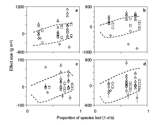
The Price Equation partition attributes the decline in total plant biomass with declining plant species richness solely to loss of plant species richness per se (the SRE) (Fig. B3). However, the SCE and CDE vary greatly among post-loss plots, at low levels of species loss the SRE generally is small relative to the SCE and CDE, and at some locations the CDE increases on average as more species are lost (Fig. B3). The net result is that total plant biomass generally declines log-linearly with declining species richness after statistically controlling for other factors. Results of conventional statistical analyses and the Price Equation partition are not contradictory. Rather, the Price Equation partition helps interpret statistical analyses in terms of effects that are well-defined outside the context of certain experimental designs.

Besides the SRE, differences in aboveground biomass between pre- and post-loss plots are attributable to the SCE and CDE. In the BIODEPTH experiment, the CDE often is larger in absolute magnitude than the SCE, or any possible SCE (Fig. B3). This indicates that which species are lost often is a less-important determinant of total biomass than the response of the remaining species. Interestingly, this response need not depend on the identity of the lost species or the remaining species. At Portugal and Sweden, mean SCE and mean CDE are uncorrelated among less-diverse plots, indicating that the identity of the lost species (and thus of the remaining species) does not determine the response of the remaining species to species loss (Table B1). At the other two sites a negative correlation between mean SCE and mean CDE indicates that loss of high-biomass species (= negative SCE) tends to lead to an increased compensatory response by the remaining species (= positive CDE). Variation among locations in the correlation between the SCE and CDE suggests that the mechanisms of interaction among plants may be location-specific to some extent.

Within each location, all of the most-diverse plots but only some of the less-diverse plots contained nitrogen-fixing legumes. It might be thought that loss of the facilitative interactions between legumes and other plants would reduce the potential for compensatory growth by the remaining species. This hypothesis predicts that post-loss plots lacking legumes will tend to have lower CDEs (and thus lower total biomass) than post-loss plots with legumes. The data reject this hypothesis: mean CDE does not depend on whether or not legumes are present in the post-loss plot, except at Sheffield (1-way ANOVAs: Sheffield, F_1,24 = 6.62, P = 0.017; other sites, P > 0.6). The significant result for Sheffield should be interpreted cautiously, because at Sheffield (and other locations) presence/absence of legumes is confounded with post-loss richness: it is largely the least-diverse plots that lack legumes. At Sheffield, omitting the 4- and 8-species post-loss plots from the analysis (none of which lacked legumes) eliminates the significant effect of legume presence/absence on mean CDE (F_1,8 = 2.96, P = 0.12).

It might be thought that an effect of legume presence/absence on the potential for compensatory growth will be obscured by context dependence generated by the substitutive experimental design (see below). However, legume presence/absence is not significantly related to CDE_p (context dependence of per-capita biomass) at any of the four locations (results not shown), and CDE_p is unaffected by the experimental design (see below).

In summary of the legume analyses, losing all legumes does not have a major impact on the potential of the remaining species for compensatory growth. This result does not contradict conventional statistical analyses that find a significant effect of legume presence/absence on total biomass (Spehn et al. 2005), because the CDE only captures some of the ecological mechanisms by which legume loss can affect total biomass, and because the CDE also incorporates effects of other ecological mechanisms unrelated to legume loss. However, results of the Price Equation partition do suggest a reinterpretation of conventional statistical results. Significant effects of the presence/absence of legumes on total biomass in conventional statistical analyses of BIODEPTH probably arise in large part simply because some legumes are among the highest-biomass species at most BIODEPTH sites, with facilitation of other species by legumes playing a lesser role.

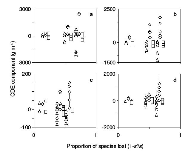
In part, the CDE reflects the substitutive experimental design, as described in the main text for the analysis of Mulder et al. (1999). Increased species abundance with decreasing post-loss richness (increased positive CDE_n, reflecting the experimental design) is associated with reduced per-capita functional contribution (negative CDE_i), as expected if species compete more intensely intra- than interspecifically (Fig. B4). CDE_p is near-zero on average at each location and typically smaller in absolute magnitude than CDE_n and CDE_i (Fig. B4), as expected if plots within locations had similar environmental conditions. In contrast, Mulder et al. (1999) found large values of CDE_p when pre- and post-loss plots differed in the presence/absence of insect herbivores (see main text).

Analysis of Ives and Cardinale (2004)

Ives and Cardinale (2004) modelled the effect of species loss on ecosystem tolerance to an environmental stressor. Ives and Cardinale (2004) described the dynamics of the species within a site using modified Lotka-Volterra equations with randomly-chosen parameter values. These equations describe how species’ equilibrium abundances depend on the trophic interactions among species as well as on an environmental stressor. The tolerance of species i to the stressor (, the functional contribution of species i) can be defined as the sensitivity of its equilibrium abundance to a small increase in the value of the stressor. The tolerance of the ecosystem as a whole (the ecosystem function of interest) can be defined as the mean sensitivity of all species, . To illustrate the application of the Price Equation partition to this model, I constructed a pre-loss site with s = 10 species, a random food web topology (as in Ives and Cardinale (2004)), and the parameter p (which scales the magnitude of interspecific interactions relative to intraspecific interactions) set to 1. I then removed the species with the lowest tolerance and recalculated the tolerances of the remaining species using the analytical formulae in Ives and Cardinale (2004) to obtain post-loss values. Iterating this procedure generated a series of post-loss sites with species, each of which was compared to the pre-loss site using the Price Equation partition of (bracketed term in equation (4)).

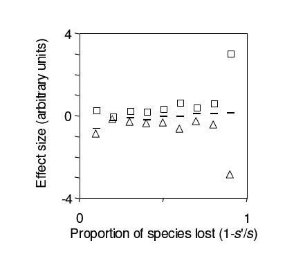
Since the ecosystem function of interest is rather than T, both the SCE and CDE are unscaled by post-loss richness (see bracketed terms in equation (4)). Since both terms are unscaled, both are inversely related to the proportion of species remaining, and so increase in absolute magnitude as a greater proportion of species are lost, other things being equal (Fig. B5). Under the assumptions of Ives and Cardinale (2004), the unscaled CDE and unscaled SCE are approximately equal in magnitude but opposite in sign, so that mean tolerance varies little with species loss (dashes in Fig. B5).

TABLE B1. Correlations between the mean values of SRE or SCE, and CDE, for less-diverse plots within each location of the BIODEPTH experiment (Spehn et al. 2005).

   Notes: Use of means avoids non-independence that would arise from using all pairwise comparisons between pre- and post-loss plots. n is sample size (number of less-diverse plots with ≥2 species), r values are Pearson’s correlation coefficients with subscripts indicating the two components of the Price Equation partition being correlated. *P < 0.05, ***P < 0.001.

FIGURES

FIG. B1. Effects of species loss on ecosystem function in different studies, vs. proportion of species lost. In both panels, the mean SRE (diamonds), mean SCE (squares), and mean CDE (triangles) for each “post-loss” site are shown. Error bars (many of which are zero or too small to display) indicate ±1 SE and reflect variation among the pre-loss sites to which the post-loss site is compared. Some points coincide; some are jittered horizontally for clarity. (a) Effects on total aboveground plant biomass on islands (sites) (Wardle et al. 1997). (b) Effects on total abundance of soil nematodes in different areas (sites) (Belnap et al. 2005). Sites are either uninvaded by an exotic plant (the “pre-loss” site), or recently or historically invaded (the two “post-loss” sites, with the historically invaded site having a greater proportion of species lost).

FIG. B2. Predictors of effect sizes in Wardle et al. (1997). (a) Partial regression of mean SCE for each “post-loss” island on the mean difference between “pre-loss” and “post-loss” soil N, after statistically controlling for other effects. (b) Partial regression of mean CDE for each “post-loss” island on mean SCE, after statistically controlling for other effects.

FIG. B3. Effects of species loss on total aboveground plant biomass (g/m2) in four locations ((a) Silwood; (b) Sheffield; (c) Portugal; (d) Sweden) from the third year of the BIODEPTH experiment (Spehn et al. 2005), vs. proportion of species lost. Within each location, sites (experimental plots) varied in species richness and composition. Symbols and error bars as in Fig. B1. See text for details.

FIG. B4. Subcomponents of the CDE at four locations ((a) Silwood; (b) Sheffield; (c) Portugal; (d) Sweden) from the third year of the BIODEPTH experiment (Spehn et al. 2005), vs. proportion of species lost. Each panel shows the average magnitude of the CDEn (diamonds), CDEp (squares), and CDEi (triangles) for each less-diverse (“post-loss”) experimental plot. Error bars as in Fig. B1. Some points are slightly jittered horizontally for clarity. See text for details.

FIG. B5. Effects of species loss on mean tolerance to a stressor in the model of Ives and Cardinale (2004). Species were lost one at a time, starting with the least-tolerant; after species loss the tolerances of the remaining species were recalculated and the procedure repeated. Dashes give the difference between mean post-loss tolerance and mean pre-loss tolerance vs. proportion of species lost. Squares (unscaled SCE) and triangles (unscaled CDE) show the two additive components of . See text for details.

LITERATURE CITED

Belnap, J., S. L. Phillips, S. K. Sherrod, and A. Moldenke. 2005. Soil biota can change after exotic plant invasion: does this affect ecosystem processes? Ecology 86:3007–3017.

Hector, A., M. Loreau, B. Schmid, and the BIODEPTH Project. 2002. Biodiversity manipulation experiments: studies replicated at multiple sites. Pages 36–46 in Loreau, M., S. Naeem, and P. Inchausti, editors. Biodiversity and ecosystem functioning. Oxford University Press, Oxford, UK.

Ives, A. R., and B. J. Cardinale. 2004. Food-web interactions govern the resistance of communities after non-random extinctions. Nature 429:174–177.

Mulder, C. P. H., J. Koricheva, K. Huss-Danell, P. Höberg, and J. Joshi. 1999. Insects affect relationships between plant species richness and ecosystem processes. Ecology Letter 2:237–246.

Spehn, E. M. et al. 2005. Ecosystem effects of biodiversity manipulations in European grasslands. Ecological Monographs 75:37–63.

Stewart-Oaten, A. 1995. Rules and judg[e]ments in statistics: three examples. Ecology 76:2001–2009.

Wardle, D. A., O. Zackrisson, G. Hornberg, C. Gallet. 1997. The influence of island area on ecosystem properties. Science 277:1296–1299.