There is no easy answer to the first question, because there are an infinite number of resource axes that could be partitioned by species. If two species show complete overlap in niche characteristics, there is always the possibility that partitioning occurs along another, unmeasured axis. However, Schoener (1974) argued that microhabitat, diet, and temporal activity time are the three most important niche axes, and that most differentiation occurs along the first two of these axes.
To address the second question, MacArthur and Levins (1967) introduced the first index of niche overlap, which was based on the relative utilization of different segments of a niche resource axis, and how much overlap there was between species in their use of common segments. MacArthur and Levins (1967) explicitly related this niche overlap index to the competition coefficients of the Lotka Volterra equation in order to derive ecological limits to the similarity of competing species.
A variety of indices have been proposed since then, which can be calculated for field measurements of the ecological niche such as utilization of dietary components, microhabitat, or temporal or spatial activity. The indices typically range from 0 (no resources used in common between two species) to 1.0 (complete overlap in resource use).
However, all of these indices are sensitive to the number of species and niche categories compared, and they may give counterintuitive results as different species or resource states are added or deleted from the data (Feinsinger et al. 1981). For these reasons, comparison with an appropriate statistical model is essential.
The third question– how much niche overlap would be expected in the absence of competition– epitomizes the null model approach. It is not enough to show that species differ in their use of resources in a way that reduces niche overlap. Even in the absence of competition, species will differ in their utilization of resources (Connell 1980).
Schoener (1974) suggested that niche overlaps observed in nature were less than expected by chance, and Sale (1974) and Inger and Colwell (1977) provided the first null model tests of this hypothesis. Lawlor (1980) developed the randomization algorithms (RAs) that are commonly used, and Haefner (1988) and Winemiller and Pianka (1990) systematically compared the power of different niche overlap indices and randomization algorithms. This module of EcoSim lets you carry out these simulations with your own data.
If you were studying lizard behavior, each column might represent the different micro-habitats that species used for perches (tree trunks, tree limbs, open ground). The categories can be either ordered or unordered. For ordered categories, you may wish to examine the size overlap module, which can be used to analyze the overlap of body sizes, flowering peaks, or peaks in other continuously measured niche data.
For the niche overlap module, the entries in each cell represent the observed utilization of the resource by a particular species. Depending on your categories, these entries might be counts, biomasses, activity times, or percentages. EcoSim will accept any non-negative real number as valid input for this module. Your data set will probably also contain some zeroes, which represent niche categories that were not utilized by a particular species. These zeroes are important because they are treated differently in the different randomization algorithms.
Winemiller and Pianka (1990) have systematically compared the behavior of 4 randomization algorithms (RA1, RA2, RA3, RA4) used in the analysis of niche overlap, and their paper should be consulted for more details. EcoSim allows you to specify these 4 algorithms (plus others) by controlling how EcoSim handles niche breadth and zero states in the matrix.
The default value for niche breadth is "retained" and the default value for zero states is "reshuffled". These defaults produce RA3. In this randomization algorithm, the niche utilization values are reshuffled within each row of the matrix. Winemiller and Pianka (1990) have shown that RA3 has good statistical properties for detecting non-random niche overlap patterns.
The default value for resource states is "equiprobable", so the different resource states are assumed to be equally abundant in the environment.
Both of these indices are also symmetric. In other words the overlap of species 1 on species 2 is equivalent to the overlap of species 2 on species 1. Fewer calculations are required using these indices, although they may not reflect asymmetric competitive effects of species on one another.
Both indices are calculated for a set of j = 1 to n resource states. Let p1j = the proportional use of resource state j by species 1. These proportional values are calculated in EcoSim by summing up the row totals, and then dividing each entry in the matrix by its row sum. Therefore, the pijs will sum to 1.0 for each species. EcoSim always takes the data and rescales it in this way before any indices are calculated or any randomizations are carried out. Once the data have been rescaled, EcoSim will calculate the overlap between every pair of species in the assemblage.
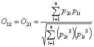
Pianka index For species 1 and 2, with resource utilizations p1i and p2i, Pianka´s (1973) overlap index of species 1 on species 2 (O12) is calculated as:
|
This index is similar to the original asymmetric MacArthur and Levins (1967) index. The denominator has been normalized to make it symmetric, but the stability properties are unchanged (May 1975).
Czechanowski index For species 1 and 2, with resource utilizations p1i and p2i, the Czechanowski index is:
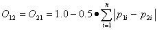 |
Graphically, this index corresponds to the area of intersection of the utilization histograms of the two species. Like the Pianka index, it is symmetric and ranges from a minimum of 0 to a maximum of 1.0.
The other choice is to relax the observed niche breadth. In this option, the observed utilization is replaced by a uniform 0-1 value, so that all utilization levels are equiprobable for any resource. This usually leads to a much broader utilization spectrum, and hence greater niche overlap, in the simulated versus the real community.
The alternative choice (which is the default option) is for the zero states to be reshuffled. In this case, resource states that were not used by a species in nature could be utilized in the null communities.
Retaining the zero structure would be important if you felt the zeroes represented utilization constraints that were imposed by forces other than species interactions. Do you think the species in your assemblage could have used any of the possible resource categories in the absence of interspecific competition? If so, you should reshuffle the zeroes in the null community. On the other hand, if you believe that certain categories be unusable even if there were no other species were present, you should retain the zero states (or use the hard zeroes option, described below)?
RA1: Niche breadth relaxed/Zero States reshuffled RA1 replaces every cell in the matrix with a randomly chosen, uniform number between zero and 1. This eliminates all zeros, so that all species in the pseudo-community will utilize all resource categories. RA1 destroys all structure in the matrix. It generates pseudo-communities with a high overlap and a small variance in overlap (e.g., Kobayashi 1991, Field 1992). Because it generates all possible assemblages of generalists, RA1 is "too null" and probably should not be used for published comparisons with real communities. NOT RECOMMENDED.
RA2: Niche breadth relaxed/Zero States retained RA2 also substitutes a random uniform number for utilizations, but it is more realistic because it retains the zero structure of the matrix. It is a useful algorithm when you believe that, in the absence of species interactions, certain resource states are unavailable for each species, but there are no other constraints on resource utilization. We recommend it as an alternative to RA3 for cases in which you want to retain the zero structure of the data.. RECOMMENDED.
RA3: Niche Breadth retained/ Zero States reshuffled RA3 retains the niche breadth of each species, but randomizes which particular resource states are utilized. It corresponds to a simple reshuffling of each row of the matrix. Use RA3 when you want to retain the amount of specialization for each species, but allow it to potentially use other resource states. Winemiller and Pianka (1990) compared the behavior of RA3 and RA4 and found that RA3 was usually superior in detecting non-random overlap patterns. We recommend it as the default choice if you aren´t sure which algorithm would be best. RECOMMENDED.
RA4: Niche Breadth retained/ Zero States retained RA4 also retains the niche breadth of each species, but in addition, it fixes the zero states to their observed values. Thus, only non-zero values are reshuffled within each row. Winemiller and Pianka (1990) found that RA4 closely mimicked the structure of the real data, and did not always detect non-randomness in cases that RA3 did. Thus, it is subject to Type II error, and is a bit too conservative for general use. On the other hand, if the patterns are significant with RA4, they are probably quite strong. NOT RECOMMENDED.
Data-defined This option instructs EcoSim to divide each observation in the observed data matrix by the column total in the matrix. Without any independent estimates of resource availability, we assume that the availability of different resource states is proportional to the column totals of the matrix. Lawlor (1980) suggested that scaling the observed utilization matrix in this way produces a matrix of electivities, which more directly reflect the niche characteristics of a species. Lawlor (1980) argued that electivities are more appropriate for analyzing patterns of niche overlap, because utilization values reflect both the electivity of the species for the resource and the availability of that resource. The scaling of the observed utilization matrix is done only once, at the start of the analysis. All randomizations and comparisons are then made with the rescaled matrix of electivities.
User-defined A weakness of the equiprobable assumption is that observed niche overlap estimates may be distorted if some resource categories are very common and others are very rare. Lawlor (1980) argued that niche overlap analyses should be based on a matrix of electivity values, rather than utilization values. The electivity index is defined as:
 |
where Rj is a measure of the availability of resource state j. Examples might include standardized sampling of a prey community, or estimates of the relative areas of different microhabitats. These measures should be independent of your observations of the actual predator diets or microhabitat use.
If you have such measures, you can take advantage of the user-defined option. When this option is chosen, a new data window appears, with a cell for each column of the matrix. You need to enter your measure of the relative availability of each resource state in these cells. Your measure of resource availability must be a positive (non-zero) real number. Negative values, zeroes, and missing values are not allowed in this analysis. The default values given in the matrix are all 1.0, which produces a null model in which all resource states are equally common. EcoSim rescales the observed matrix by dividing each utilization value by the estimate of resource availability that you provided. All analyses are then carried out on this modified matrix.
Lawlor (1980) originally suggested that electivities could be calculated by scaling the observed utilization matrix to the column totals of the matrix itself. That is, the relative resource availability could be estimated from the utlization data directly (Colwell and Futuyma 1971). Previous versions of EcoSim allowed for this rescaling option. However, we have since discovered that this approach leads to Type I errors: even with a random data set, rescaling to the column totals often generates a statistically significant patterns. Thus, some independent estimate of resource availability is necessary to move beyond the default assumption of equiprobable resource states. If you have such an estimate, EcoSim allows you to incorporate the data with the user-defined option.
Unlike most of the simulation options in EcoSim, the hard zeroes option is not invoked from the preferences menu. Instead, you create hard zeroes by entering an "x" or "X" in your data matrix. EcoSim recognizes these x's in niche overlap as hard zeroes and will not reshuffle them in the simulation. In both the real and the simulated matrices, x's are treated as zeroes in the calculation of niche overlap metrics. Thus, everywhere that an x appears in your matrix, a zero will appear in the simulated matrix. If you have ordinary zeroes in your matrix, they will be reshuffled and may be replaced or moved around in the simulated communities.
The hard zeroes option should be used only in conjunction with the Zero States | Reshuffled option. If you selected Zero States | Retained, none of the zeroes or x's would be reshuffled in the null communities.
This new feature allows the user to incorporate additional biological information and tailor the constraints to each individual species. For example, in an analysis of dietary overlap, you could use hard zeroes to fix dietary categories that a particular species could never use –whether or not other species were present– because of morphological constraints.
Hard zeroes could also be used to set realistic phylogenetic limits in the analysis of niche overlap. For example, in a study of phenological niche overlap, the user could set the limits for each species based on known flowering times for other species in the genus (e.g., Kochmer and Handel 1986). In this case, hard zeroes would represent flowering times for each species that were outside the limits of its genus.
Another possibility is that hard zeroes could be adapted to the analysis of the spatial overlap of organisms in an ecological gradient. For example, each row could represent a different inter-tidal algal species and each column could represent a different tidal height. The entries would be the densities of each species at each tidal height (Colman 1933).
A common paradigm in intertidal ecology is that the upper limits of distribution are set by abiotic factors and the lower limits are set by biotic interactions (Connell 1975). The prediction is that the overlap in densities is less than expected by chance, given that species occur independently of one another, but their upper boundaries are set by abiotic factors.
Hard zeroes could be used for a realistic test of this hypothesis, by replacing with 'x's all the zeroes that are above the highest intertidal occurrence of each species. Other zeroes in the matrix are left unchanged, because they could contain positive densities in the randomly constructed assemblages (We thank Aaron Ellison for requesting this feature and suggesting this example).
Finally, hard zeroes could be used with experimental data in which an investigator manipulates resource utilization of one or more species. If you use your imagination, you will find many uses for this new EcoSim option.
The next three panels form the histogram window. The first two columns give the lower and upper boundaries for 12 evenly spaced histogram bins. The integer number in the last column on the right tells you how many of the simulated means fell into the bin. These integers sum up to the total number of iterations that were specified for the run.
The placement of the observed mean shows you, graphically, where the observed mean fell in the histogram distribution. You can use these data to plot the histogram and the observed value if you want to illustrate your results with a graph.
The lower panel gives the mean and variance of the average niche overlap in the simulated communities. It then tells you the tail probability that the observed mean overlap was greater than or less than expected by chance.
The traditional interpretation of these patterns has been that a significantly small observed overlap implies interspecific competition and resource partitioning, whereas a significantly large overlap might indicate shared resource utilization and a lack of competition (Gotelli and Graves 1996). However, it is also possible that high overlap implies strong competition that has not yet led to divergence in resource use. Either scenario is possible, and additional data on resource availability and species interactions is necessary for a definitive answer (Sale 1974, Connell 1980). The null model tests can at least indicate which direction the patterns are in.
The placement of the observed variance shows you, graphically, where the observed variance fell in the histogram distribution. You can use these data to plot the histogram and the observed value if you want to illustrate your results with a graph.
The lower panel gives the mean and variance of the average niche overlap in the simulated communities. It then tells you the tail probability that the observed mean overlap was greater than or less than expected by chance.
An unusually small variance might characterize a community in which species number is maximized through diffuse competition and a limit to similarity. A high variance in resource use might indicate some internal guild structure, in which some species pairs are very similar in resource use and others are very dissimilar (Winemiller and Pianka 1990). Alternatively, means and variances in resource overlap could reflect the availability and suitability of difference resource states, and need not imply competitive effects (Bradley and Bradley 1985).
These models all assume that the different resource states are equi-probable. If this is not true, using observed utilizations biases the tests finding greater overlap than expected. If resource availabilities are known or can be estimated, it is more appropriate to analyze a species electivity, calculated as:
|
Where eij is the electivity ("preference") of species i for resource j, pij is the utilization of resource j by species i, and Rj is the relative abundance of resource state j (Lawlor (1980). If you can estimate these resource states independently, you should do so and then analyze both utilization and electivity patterns. EcoSim calculates electivities for you with the "user-defined" option for resource states.
The models also assume that the utilizations (p(ij)s) have been estimated accurately. In other words, there are no biases due to small sample sizes. For example, if you only had a single food item from the gut of one of your species, that species would always be recorded as a "specialist" no matter what its feeding preferences were. Simulations by Ricklefs and Lau (1980) suggest that at least 50 observations per species are necessary to avoid this sort of bias in niche overlap indices. However, small sample sizes are not really a problem for RA3 and RA4 because these algorithms retain the species niche breadth. Consequently, the simulation results are not distorted by any biases that may be present in the estimates of species' resource utilization.
All five species coexist in boreal forests of the northeastern U.S. They are small insectivorous species that are superficially similar in body size, morphology and feeding habits. There seemed to be few niche differences between them that could account for their coexistence. MacArthur (1958) carefully observed the amount of time that individuals of each species spent foraging in different parts of the trees, and argued that differences between species were sufficient to allow for species coexistence.
Use EcoSim to load the tutorial file called "MacArthur's warblers." This file has 5 rows, representing the different species. Use the mouse to drag on the column labels and expand them so you can read them. There are 16 columns (1T, 1M, 1B, and 2T…), representing different sections of the tree. Section 1 is at the crown and section 6 is at the base of the tree. T stands for "terminal", M stands for "middle", and B stands for "basal". See the figures in MacArthur´s (1958) paper for the location of these regions.
Each entry in the matrix is the percentage of time that a species spent foraging in a particular section of the tree. For example, the first cell in the matrix has the value 49.9. This means that the Cape May warbler spent 49.9% of its foraging time in the terminal region of the crown of the tree (1T). Thus, the entries in each row sum to 100 for each species.
MacArthur (1958) argued that these numbers were evidence that the species were partitioning the niche of physical space in the tree. But how much overlap would we expect if there were no interactions among these species? The simulations in EcoSim provide a number of answers to this question!
Call up the Niche Overlap module from the Analyze menu. In the random number seed box, enter the integer "10" but do not change any of the other defaults. Normally, you would use the default random number seed provided by the system clock, but in this case you want to produce precisely the same set of numbers that were used in this tutorial. Now click on the Run button and EcoSim will perform 1000 simulations of niche overlap, which should take less than 1 minute of computing time.
The Input tab shows you the original data set. Compare this matrix to the one in Simulation tab, which shows you one of the simulated matrices. You should see that the values in each row have been randomly reshuffled into different columns.
Now go to the Pairwise tab. This shows you the observed pairwise niche overlaps, calculated using Pianka´s (1973) niche overlap index. This index measures the relative amount of habitat overlap between each pair of species and ranges from a minimum of 0.0 (no shared habitats) to a maximum of 1.0 (identical habitat use). From this, you can see that the observed niche overlap in feeding position was highest between the Cape May and Blackburnian warblers (0.93), and lowest between the Cape May and Bay-breasted warblers (0.24).
Now click on the Mean tab to see some simulation results. In the left column, you will see the observed mean, which is 0.55514. This is the mean of the 10 pairwise niche overlaps that you saw in the Pairwise tab. The position of the observed mean is indicated by a text arrow, which points to a row in the histogram box. This histogram box summarizes the mean niche overlap that was found for the 1000 simulated matrices.
Notice that the observed niche overlap (0.55514) falls in the bin interval from 0.55318 - 0.58014. The 12 bin intervals are evenly spaced between the minimum and maximum of the simulated niche overlaps. The integer number to the right of the interval tells you how many of the simulated matrices fell in this bin. In this case, there were 3 simulations that fell in this interval, and 2 simulations fell in the next higher interval. The remaining 995 simulations had average niche overlaps less than this interval. These integers will always sum up to the number of iterations you have requested EcoSim to perform.
In the box below, you can read the observed mean (0.55514) and the mean (0.39138) and the variance (0.00141) of the 1000 simulated mean niche overlaps.
Next is the lower and upper tail probability. This shows that, by chance, the probability that the observed mean niche overlap was less than or equal to the expected mean is 0.995. EcoSim found that 995 of the simulated means were less than or equal to the observed mean. In contrast, only 5 out of the 1000 simulated means are greater than or equal to the observed mean. Therefore, the probability of observing, by chance, a mean niche overlap of 0.55514 or more is only 0.005.
Although MacArthur (1958) concluded that the warbler species overlapped less than expected, this analysis gives exactly the opposite result: observed niche overlap was improbably high, compared to this particular simulation! However, as we shall see, the results are sensitive to which simulation is used and how the data are treated.
Now move to the variance tab. This tab gives you the observed variance in pairwise niche overlap (0.02737) and compares it to the variance of niche overlap in the simulated matrices. In this case, the average of the simulated variances is 0.01693, and the left- and right- tail probabilities are 0.901 and 0.099, respectively. Neither of these are extreme values (< 0.05), so there is no strong evidence that the observed variance differs from chance.
The Summary tab repeats all of the information from the previous tabs, gives you the options, iterations, and random number seed that you selected and shows you a small time clock in the lower right-hand corner. You can edit or annotate all of these results and save them to a disk file if you wish.
So what have we learned?
This simulation suggests that the observed variance is not statistically different from the null model, but the observed mean and median niche overlap are significantly greater than expected by chance.
However, the results will depend on the simulation algorithm used. Run the simulation again, using Niche Breadth | Relaxed and Zero States | Reshuffled. This is the most liberal of the 4 randomization algorithms (RA1), because it replaces every observation in the data matrix with a random, uniform number between 0.0 and 1.0.
RA1 always generates a very high expected overlap, with a small expected variance. You will see that the observed mean niche overlap is less than all of the simulated niche overlaps created by RA1, whereas the observed variance in niche overlap is larger than the variance in all of the simulated communities.
RA2 is created by using Niche Breadth | Relaxed and Zero States | Retained. RA2 replaces only the non-zero elements in the matrix with random, uniform numbers. For the MacArthur (1958) data set, RA2 generates non-significant results for the mean (p = 0.161), although the variance is significantly larger than expected (p < 0.0001).
RA4 is created by using Niche Breadth | Retained and Zero States | Retained. RA4 is similar to RA3 in that it reshuffles the data, but it only reshuffles the non-zero elements. With RA4, the observed mean niche overlap is greater than expected (p = 0.009), but the variance is marginally non-significant (p = 0.087).
In conclusion, MacArthur's (1958) claim that these warblers exhibit reduced niche overlap in foraging is supported only in comparison with RA1, which generates a "super generalist" forager for the null communities. More realistic null models suggest that niche overlap in this system is either random or higher than expected by chance. However, these conclusions depend on the assumption that resource states are equiprobable, and with independent estimates of resource availability, the results could be different.
Read the help sections on the different algorithms and some of the original literature to decide which simulation options you should be using with your own data.
Bulmer, M.G. 1974. Density-dependent selection and character displacement. The American Naturalist 108: 45-58.
Colman, J. 1933. The nature of the intertidal zonation of plants and animals. Marine Biological Association of the United Kingdom 18: 435-476.
Colwell, R.K. and D.J. Futuyma 1971. On the measurement of niche breadth and overlap. Ecology 52: 567-576.
Connell, J.H. 1975. Some mechanisms producing structure in natural communities: a model and evidence from field experiments. pp. 460-490 in: Ecology and Evolution of Communities. M.L. Cody and J.M. Diamond (eds). Harvard University Press, Cambridge.
Connell, J.H. 1980. Diversity and the coevolution of competitors, or the ghost of competition past. Oikos 35: 131-138.
Feinsinger, P., E.E. Spears and R.W. Poole. 1981. A simple measure of niche breadth. Ecology 62: 27-32.
Field, J. 1992. Guild structure in solitary spider-hunting wasps (Hymenoptera: Pompilidae) compared with null model predictions. Ecological Entomology 17: 198-208.
Gotelli, N.J. and G.R. Graves. 1996. Null models in ecology. Smithsonian Institution Press, Washington, DC.
Haefner, J.W. 1988. Niche shifts in greater Antillean Anolis communities: effects of niche metric and biological resolution on null model tests. Oecologia 77: 107-117.
Inger, R.F. and R.K. Colwell. 1977. Organization of contiguous communities of amphibians and reptiles in Thailand. Ecological Monographs 47: 229-253.
Kobayashi, S. 1991. Interspecific relations in forest floor coleopteron assemblages: niche overlap and guild structure. Researches on Population Ecology 33: 345-360.
Kochmer, J.P. and S.N. Handel. 1986. Constraints and competition in the evolution of flowering phenology. Ecological Monographs 56: 303-325.
Lawlor, L.R. 1980. Structure and stability in natural and randomly constructed competitive communities. The American Naturalist 116: 394-408.
MacArthur, R.H. 1958. Population ecology of some warblers of northeastern coniferous forests. Ecology 39: 599-619.
MacArthur, R. and R. Levins. 1967. The limiting similarity, convergence, and divergence of coexisting species. The American Naturalist 101: 377-385.
May, R.M. 1975. Some notes on estimating the competition matrix, a. Ecology 56: 737-741.
Pianka, E.R. 1973. The structure of lizard communities. Annual Review of Ecology and Systematics 4: 53-74.
Rathcke, B.J. 1984. Patterns of flowering phenologies: testability and causal inference using a random model. pp. 383-396 in: Ecological Communities: Conceptual Issues and the Evidence. D.R. Strong, Jr., D. Simberloff, L.G. Abele, and A.B.Thistle (eds). Princeton University Press, Princeton.
Ricklefs, R.E. and M. Lau. 1980. Bias and dispersion of overlap indices: results of some Monte Carlo Simulations. Ecology 6: 1019-1024.
Sale, P.F. 1974. Overlap in resource use, and interspecific competition. Oecologia 17: 245-256.
Schoener, T.W. 1974. Resource partitioning in ecological communities. Science 185: 27-39.
Winemiller, K.O. and E.R. Pianka. 1990. Organization in natural assemblages of desert lizards and tropical fishes. Ecological Monographs 60: 27-55.