Ecological Archives A025-122-A2
Erik R. Schoen, David A. Beauchamp, Anna R. Buettner, and Nathanael C. Overman. 2015. Temperature and depth mediate resource competition and apparent competition between Mysis diluviana and kokanee. Ecological Applications 25:19621975. http://dx.doi.org/10.1890/14-1822.1
Appendix B. Hydroacoustics analysis: detailed methods, kokanee density and abundance, and vertical distribution of kokanee and Mysis.
We conducted hydroacoustic surveys at night during February, May, August, and November, 2005. Each survey consisted of 22 transects in a zig-zag pattern (Simmonds and MacLennan 2005). We used a Biosonics DE 6000 echosounder and a 200-kHz split-beam transducer with a 6.7° beam width. We used a target-strength threshold of -55 dB, allowing detection of fish as small as 30 mm total length (Love 1971). We conducted supplemental short transects in conjunction with each Mysis haul to determine the vertical distribution of Mysis. We used a target-strength threshold of -70 dB for Mysis transects, a compromise level that allowed us to detect the Mysis scattering layer as deep at 100 m, although it was not sensitive enough to detect individual mysids (Rudstam et al. 2008). We recorded the upper and lower limits of the continuous Mysis scattering layer in these echograms. We followed the hydroacoustic data acquisition methods and stratified statistical design of Schoen et al. (2012) for the kokanee surveys. We estimated kokanee density by echo counting single acoustic targets with Echoview version 4.2 software (Myriax Pty). Kokanee were dispersed from schools during the night-time surveys and relatively low in density (August mean density = 46.6 kokanee / ha), justifying this approach (Rudstam et al. 2012). We excluded data collected within 4 m of the transducer face from the analysis due to near-field distortion and the potential for boat avoidance (Rudstam et al. 2012). We assumed that all small (< 330 mm FL), pelagic targets (> 5 m above the lake bottom) were kokanee because kokanee comprised 95% of the mid-water gill net catch and modal sizes of acoustic targets corresponded with the size distribution of kokanee. We used size modes of hydroacoustic targets to assign targets to kokanee age classes.
We estimated the areal density of kokanee in each lake basin, partitioned by age class and season. We converted density to abundance by multiplying by the surface area of the pelagic zone (defined here as bottom depth > 15 m) of each basin (Kendra and Singleton 1987). The August survey was conducted under optimal conditions for determining kokanee abundance, on moonless nights during peak thermal stratification (Beauchamp et al. 2009). During the other months, kokanee were only partially detectable due to a shallower distribution and greater potential for boat avoidance. Thus, we used the August survey to determine the absolute abundance of kokanee, and we used the February, May, and November surveys to quantify seasonal changes in relative abundance between lake basins. We then estimated the absolute abundance of kokanee during February, May, and November by adjusting the August abundance to account for mortality (see below) and partitioning the lake-wide population between basins using the relative abundances determined in the seasonal surveys. We quantified the uncertainty in the density, abundance, and survival estimates with 95% BCa bootstrapped confidence intervals calculated in R with the ‘boot’ package (Canty and Ripley 2014).
We estimated age-specific kokanee survival rates from our hydroacoustic data and the literature. We estimated the annual survival rate of age-0 and age-1 kokanee based on the ratio of these age classes detected in the August 2005 hydroacoustic survey. We assumed recruitment of these cohorts was nearly equal (Miranda and Bettoli 2007), which was reasonable because similar numbers of kokanee spawned in the 2003 and 2004 brood years (5% difference; Schoen and Beauchamp 2010) and similar numbers of age-0 kokanee were stocked in 2004 and 2005 (7% difference; Keesee and Keller 2013). We estimated an annual survival rate S = 49.5% (95% CI: 43.8–60.4%; instantaneous annual mortality rate Z = 0.703, 95% CI: 0.505–0.826) for age-0 and age-1 kokanee. This was similar to survival rates reported for juvenile kokanee in other lakes (reviewed by McGurk 1999). We used literature data to estimate the survival of older kokanee age classes. The hydroacoustics data were not suitable for estimating survival of the age-2 and older cohorts because their size modes overlapped and spawner numbers varied substantially between their respective brood years, violating the assumption of equal recruitment. Instead, we estimated the survival rate of kokanee 2 years and older as 33% (Z = 1.11 ± 0.133 / yr; mean ± SE), the survival rate reported for 48 brood years of age 2-3 kokanee across eight other lakes (McGurk 1999). To incorporate uncertainty in this literature-based survival rate into our abundance calculations, we randomly drew a value of Z from a normal distribution with the above parameters for each bootstrapped simulation.
Literature Cited
Beauchamp, D. A., D. Parrish, and R. A. Whaley. 2009. Salmonids/coldwater species in large standing waters. Pages 97–117 in S. Bonar, D. W. Willis, and W. A. Hubert, editors. Standard Sampling Methods for North American Freshwater Fishes. American Fisheries Society, Bethesda, Maryland, USA.
Canty, A., and B. Ripley. 2014. boot: Bootstrap R S-Plus) Functions. R package version 1.3-11.
Keesee, B. G., and L. M. Keller. 2013. Lake Chelan kokanee spawning ground surveys 2012. Final report. Chelan County Public Utility District, Wenatchee, Washington, USA.
Kendra, W., and L. R. Singleton. 1987. Morphometry of Lake Chelan. Water Quality Investigations Section, Washington State Dept. of Ecology, Olympia, Washington, USA.
Love, R. 1971. Dorsal aspect target strength of an individual fish. The Journal of the Acoustical Society of America 49:816.
McGurk, M. D. 1999. Size dependence of natural mortality rate of sockeye salmon and kokanee in freshwater. North American Journal of Fisheries Management 19:376–396.
Miranda, L. E., and P. W. Bettoli. 2007. Mortality. Pages 229–277 in C. S. Guy and M. L. Brown, editors. Analysis and Interpretation of Freshwater Fisheries Data. American Fisheries Society, Bethesda, Maryland, USA.
Rudstam, L. G., J. M. Jech, S. L. Parker-Stetter, J. K. Horne, P. J. Sullivan, and D. M. Mason. 2012. Fisheries acoustics. Pages 597–636 in A. V. Zale, D. Parrish, and T. M. Sutton, editors. Fisheries Techniques, Third edition. American Fisheries Society, Bethesda, Maryland, USA.
Rudstam, L. G., F. R. Knudsen, H. Balk, G. Gal, B. T. Boscarino, and T. Axenrot. 2008. Acoustic characterization of Mysis relicta at multiple frequencies. Canadian Journal of Fisheries and Aquatic Sciences 65:2769–2779.
Schoen, E. R., and D. A. Beauchamp. 2010. Predation impacts of lake trout and Chinook salmon in Lake Chelan, Washington: Implications for prey species and fisheries management. Washington Cooperative Fish and Wildlife Research Unit, U.S. Geological Survey, University of Washington, Seattle, Washington, USA.
Schoen, E. R., D. A. Beauchamp, and N. C. Overman. 2012. Quantifying latent impacts of an introduced piscivore: Pulsed predatory inertia of lake trout and decline of kokanee. Transactions of the American Fisheries Society 141:1191–1206.
Simmonds, J., and D. MacLennan. 2005. Fisheries Acoustics: Theory and Practice. Second edition. Blackwell Science, Oxford, UK.
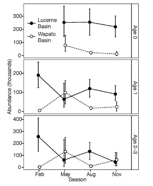
Fig. B1. Typical vertical distributions of kokanee and Mysis at night in Lucerne and Wapato Basins (August 2005 distributions depicted here). Kokanee and Mysis distributions were determined from hydroacoustic surveys. Dashed lines represent the vertical extent of the Mysis scattering layer viewed on hydroacoustic echograms. Solid curves represent thermal profiles. In both basins, kokanee were distributed both above and below the thermocline, while Mysis were restricted to deeper waters cooler than 14° C.
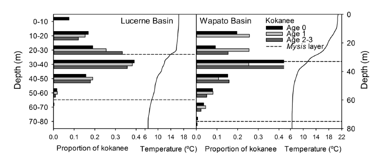
Fig B2. Seasonal kokanee abundance in Lucerne and Wapato Basins as estimated from hydroacoustic surveys. Error bars represent 95% bootstrapped confidence intervals. Values are slightly shifted horizontally to show overlapping points.