Ecological Archives A025-107-A1
Alison Johnston, Daniel Fink, Mark D. Reynolds, Wesley M. Hochachka, Brian L. Sullivan, Nicholas E. Bruns, Eric Hallstein, Matt S. Merrifield, Sandi Matsumoto, and Steve Kelling. 2015. Abundance models improve spatial and temporal prioritization of conservation resources. Ecological Applications 25:17491756. http://dx.doi.org/10.1890/14-1826.1
Appendix A. Extended descriptions of the data sources, data processing, STEM modeling framework, and local occurrence and abundance models.
Data sources and data preparation
We used abundance data from the publically available eBird Reference Dataset 5.0 (Munson et al. 2013). Checklists used for analysis were from observation periods between Jan 1st 2007 and December 31st 2012 in California, with data collected using either the “stationary count” or “traveling count” protocol. We used only “complete checklists” which are defined by the participants as a complete record of all of the species they detected and were able to identify. For all counts, data were only used from checklists with start times falling between 5am and 8pm (i.e. likely daylight hours), and the total search times of ≤3 hours; additionally, for travelling counts transect distances were limited to ≤5 miles. The resultant data set consisted of 232,175 checklists within the state of California. Each species model was trained based on 209,044 checklists and approximately ten percent of data; 23,131 checklists, were held aside for independent model validation.
All models of occurrence and abundance used the same suite of covariates (i.e., predictor variables) described here: effort covariates describing the observation process, and spatial and temporal covariates describing the ecological process. There were four effort variables associated with each checklist: the duration spent searching for birds, whether the observer was stationary or travelling, the distance traveled during the search, and the number of people in the observation group. These covariates were included in the models to account for variation in detectability associated with search effort. Elevation and land cover were included as environmental covariates. Elevation data were from the ASTER GDEM data product version 2 (Tachikawa et al. 2011) and elevation for each checklist was taken from the 30m pixel in which each checklist was located. Land cover data were from the Cropland Data Layer (USDA-NASS 2013) and were summarized within a 3km × 3km square centered on the location of each checklist. The percentage cover of each of 131 crop types were calculated using FRAGSTATS (McGarigal et al. 2012) using the data from the year in which the checklist was conducted. Time was included at two scales: the time of day, capturing differences in behavior of birds and availability for detection, and the day of the year, describing seasonal trends including migratory bird movements.
Overall STEM framework
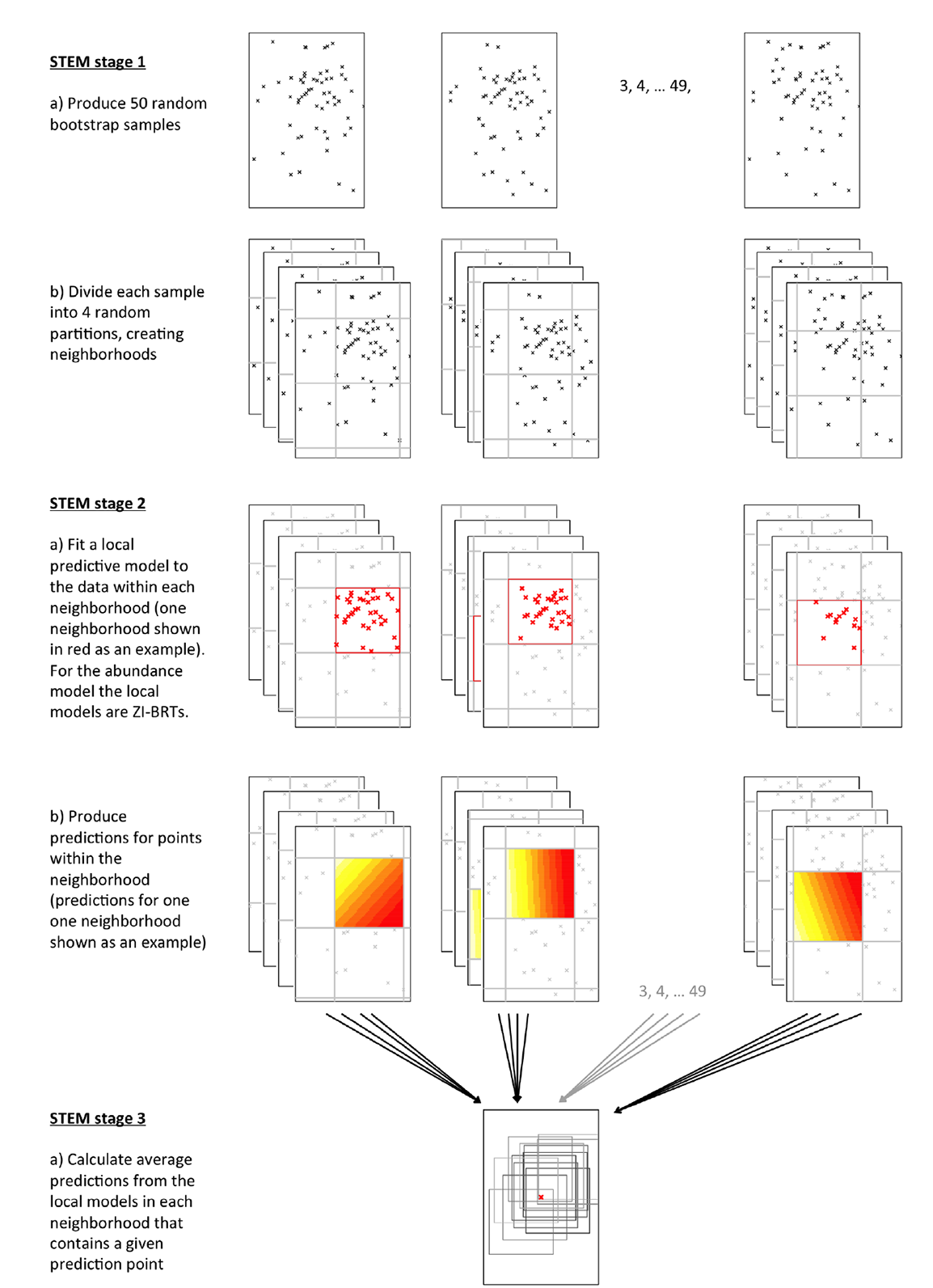
The STEM framework (Fink et al. 2010, 2014) was designed to discover scale-dependent, nonstationary covariate-response relationships from large, irregularly distributed observational data. The STEM framework is a three-stage modeling strategy (Fig. A1); first, the study extent was partitioned into several overlapping spatiotemporal neighborhoods. Second, within each neighborhood, species’ occurrence and abundance was assumed to be stationary and we constructed a local model to estimate covariate effects. Third, a mixture model was used to aggregate overlapping local neighborhood models to produce ensemble estimates of occurrence and abundance. Below we describe the local neighborhood models for occurrence and abundance (stage 2) and then we describe the partition to create the local neighborhoods (stage 1) and aggregation of local predictions (stage 3).
Fig. A1. Schematic representation of the STEM model framework. This diagram shows a spatial grid, however in reality this is a spatio-temporal grid partition. Local neighborhoods are therefore local in time as well as space. This framework is applied once using the occurrence BRT as the local model to produce estimates of occurrence. Then framework is applied a second time using the abundance ZI-BRT as the local model produces estimates of abundance.
Local Occurrence models with Boosted Regression Trees
Boosted Regression Trees (BRTs) were used to fit models to data within local neighborhoods that were defined for the STEM mixture (Fig. A1). Within each grid cell with at least 30 checklists, we fit an occurrence BRT model, which we refer to as the “local” model. BRTs are a flexible, highly automated nonparametric regression technique (Hastie et al. 2009) that can accommodate a wide-range of potential covariates with non-linear effects (De’ath and Fabricius 2000). With these characteristics, BRTs have been found to perform well for species distribution modeling (Elith et al. 2008). BRT occurrence models were fit by using presence or absence of species on a checklist as the binomial response variable (Ridgeway 2013). Effort and time covariates were included to account for variation in detectability and availability for detection of birds.
Local Abundance Models with Boosted Regression Trees
Abundance models were also fit to data within local neighborhoods (Figure S1) using BRTs, but the count response variable was more challenging to characterize statistically. Counts from wildlife surveys often have very large numbers of zero counts that arise from several distinct processes (here locations refers to location of the survey in both space and time):
These sources of zero are all particularly relevant with a broad scale citizen data set such as eBird. There will likely be many surveys that are in unoccupied locations (zeros from process 1), as participants survey a broad range of sites across the entire year. Variation in availability (zeros from process 2) is important because searches often occur at times when birds are unlikely to be present or active; thus, even searches conducted in habitat that support high population densities may not coincide with the presence or high counts of the species. Detectability (zeros from process 3) may be a factor in closed habitats or poor weather, but citizen science projects have another source of variation in detectability – variation in the expertise and skill of the participants in detecting and identifying species.
For each local neighborhood model we used a two-step Zero-inflated Boosted Regression Tree (ZI-BRT) to account for excess zero counts when modeling species abundance. The first step of the ZI-BRT was a binary response BRT used to distinguish between suitable and unsuitable habitats, the largest source of excess zeros when modeling eBird data across broad extents. This stage was very similar to the BRT occurrence model, but to account for the fact that higher observed abundances describe more suitable habitat, the binomial likelihood function used to fit the BRT was weighted by the square root of the observed abundance plus one.
The second step of the ZI-BRT used a Poisson response BRT to estimate abundance based on the observed checklist counts. To control the number of excess zeros only checklists from sites with suitable habitat, i.e. sites with a high probability of occurrence were used to fit the model. The predicted probabilities from the first step model were used to identify these sites. The probabilities were calibrated to ensure that they matched observed frequencies of occurrence (Pearce and Ferrier 2000) (see below) and a threshold was calculated to select the sites. Those checklists that had a probability of occurrence that was greater than the calibrated threshold were selected for abundance modeling. Covariates were the same effort, time, and environmental covariates described above. Processes (2) and (3) above which lead to excess zeros can also lead to low counts of abundance, due to reduced availability for detection (caused in part by the local-scale dynamics of flocking birds moving around a landscape) and imperfect detection. To account for these low counts, the Poisson likelihood function used to fit the BRT was also weighted by the square root of the observed abundance plus one (Ridgeway 2013). Both steps of the zero-inflated abundance model included effort and time covariates to account for partial availability (process 2) and variation in detection (process 3).
To calibrate the probabilities from the first step model we used a Generalized Additive Model (GAM) describing the observed occurrence on a checklist as a smooth function of the estimated probabilities of occurrence. A logistic GAM was found to be unstable in situations of complete separation (i.e., where a single threshold of predicted probability of occurrence could completely separate presences from absences), so we used a Gaussian GAM. The smooth was given a maximum of five degrees of freedom and was constrained to be monotonically increasing (Pya 2010) and the degrees of freedom used for the smooth were selected by Generalized Cross Validation (Wood 2008). In the few cases when the GAM did not converge, it was run again with a maximum of three degrees of freedom for the smooth. Estimates from the GAM were bounded, post-hoc, to be between zero and one and the calibrated threshold for presence was calculated as the estimated probability of occurrence at which the observed frequency of occurrence was 0.5. The R package ‘scam’ was used to fit the constrained GAMs (Pya 2013). By including the calibration step within each local model in the STEM mixture, the calibration and threshold selection steps were able to adapt to spatial and temporal variation in the distribution of occurrence.
All BRTs were run with an interaction depth of three, where possible, a minimum of five checklists in each node, a shrinkage parameter of 0.01 and a bag fraction of 0.80. Where the binomial BRT model converged, but the Poisson BRT model did not converge, the Poisson BRT model was run with an interaction depth of two and a minimum of three observations in each node. If this did not converge, the estimated abundance for observations in the grid cell that that met the calibrated threshold was taken to be the median of non-zero observations in that grid cell, which is equivalent to a tree ‘stump’. This procedure created estimated abundances for grid cells with few non-zero observations, rather than biasing the results towards grid cells with many non-zero observations.
Each BRT ensemble included 1000 trees. We relied on the variance-reducing properties from averaging across the STEM mixture to control for overfitting. The trees were fit in R (R Core Team 2013) with the package “gbm” (Ridgeway 2013).
Scaling BRTs with STEM
We used the STEM model framework (Fink et al. 2010, 2014) to generate year-round predictions across the study region for each bird species. This was done separately for occurrence and abundance models.
The first stage of the STEM framework partitioned the extent of the analysis into local spatiotemporal neighborhoods (Fig. A1). In this analysis we used neighborhoods of 3˚ × 3˚ × 40 days. The second stage independently fit local models to the data within each of the neighborhoods (Fig. A1). These two stages produced 200 randomly positioned partitions (4 partitions for each of 50 bootstraps) resulting in an ensemble of partially overlapping local neighborhood models. The third stage combined this ensemble of models to create modeled predictions (Fig. A1). To make predictions at a given location and date, an average was computed across all the local models that contain the location and date. Calculating averages controls for inter-model variability and naturally adapts to non-stationary covariate-response relationships (Fink et al. 2010, 2014). In practice, STEM is defined by the neighborhood size and the method used to randomize the neighborhood partitions.
An important part of the STEM implementation was determining the size of the local neighborhoods or grid cells. A regular spatiotemporal grid with dimensions 3-degrees longitude by 3-degrees latitude by 40-days was used to partition the study area into grid cells. The size of the local grid cells controls a bias-variance tradeoff (Fink et al 2010, 2014) and must strike a balance between grid cells that are large enough to have sufficient training data (variance associated with sample size) and grid cells that are small enough to capture spatiotemporally local variation in abundance and covariate-response relationships (variability that leads to statistical non-stationarity).
Since we wanted to capture seasonal variation in distributions, we wanted the time dimension to be short enough to adapt to seasonal changes. From past experience we have found that a grid with a 40-day window can adapt to a wide variety of complex avian migration patterns across a diverse set of terrestrial species using eBird data (NABCI 2011, 2013). Day of the year was treated as circular, so that a 40-day period could stretch from December into January. The spatial dimensions were selected to be the smallest size possible (lowest bias) with the goal of capturing non-stationary patterns, but large enough to at least meet the minimum sample size requirements (variance control) for the BRTs to be fit throughout the study area (the state of California). Note that because of the sparse and irregular distribution of the eBird data, it is a non-trivial process to make this choice.
To facilitate bootstrap smoothing across neighborhoods a sample of 200 overlapping grids (3˚ × 3˚ × 40 days) was generated using a nested bootstrap design. First, 50 bootstrap samples of the data were selected to produce datasets encompassing variation in the underlying data (Fig. A1). The choice of grid starting point affects the grid partition, the division of the data and the subsequent model. Therefore, for each bootstrap sample, four randomly located grid partitions were created, to provide variation in the division of each bootstrap sample. The starting point for the grid division was randomly generated for each of the four partitions.
Central Valley Abundance and Occurrence Estimates
Abundance and occurrence were estimated across all of California, by creating predictions in a grid of standardized checklists. One random point was selected within each grid square in a 3km × 3km grid and weekly estimates of abundance and occurrence were estimated for a standardized checklist at that point. Each point was standardized to be the expected count when visited by a typical eBird participant conducting a 1km travelling count between 7am and 8am. Ensemble predictions were produced by averaging across all 200 bootstrap partitions that overlapped with a given location and time. This model averaging also acts to reduce the variance of the local models, providing a simple way to control for overfitting. Predictions from the 200 bootstrap partitions were used to produce 90% bootstrap confidence intervals.
Literature cited
De’ath, G., and K. E. Fabricius. 2000. Classification and regression trees: a powerful yet simple technique for ecological data analysis. Ecology 81:3178–3192.
Elith, J., J. R. Leathwick, and T. Hastie. 2008. A working guide to boosted regression trees. Journal of Animal Ecology 77:802–813.
Fink, D., T. Damoulas, N. E. Bruns, F. A. La Sorte, W. M. Hochachka, C. P. Gomes, and S. Kelling. 2014. Crowdsourcing meets ecology: hemispherewide spatiotemporal species distribution models. AI magazine 35:19–30.
Fink, D., W. M. Hochachka, B. Zuckerberg, D. W. WInkler, B. Shaby, M. A. Munson, G. J. Hooker, M. Riedewald, D. Sheldon, and S. Kelling. 2010. Spatiotemporal Exploratory models for Large-scale Survey Data. Ecological Applications. Ecological Applications 20:2131–2147.
Hastie, T., R. Tibshirani, and J. Friedman. 2009. The elements of statistical learning: data mining, inference, and prediction. Second edition. Springer-Verlag, New York, USA.
McGarigal, K., S. A. Cushman, and E. Ene. 2012. FRAGSTATS v4: Spatial pattern analysis program for categorical and continuous maps. University of Massachusetts, Amherst, Massachusetts, USA.
Munson, M. A., K. Webb, D. Sheldon, D. Fink, W. M. Hochachka, M. Iliff, M. Riedewald, D. Sorokina, B. L. Sullivan, C. Wood, and S. Kelling. 2013. The eBird Reference Dataset, Version 5.0. Cornell Lab of Ornithology and National Audubon Society, Ithaca, New York, USA.
NABCI. 2011. The State of the Birds 2011 Report on Public Lands and Waters. U.S. Department of Interior, Washington, DC, USA.
NABCI. 2013. The State of the Birds 2013 Report on Private Lands and Waters. U.S. Department of Interior, Washington, DC, USA.
Pearce, J., and S. Ferrier. 2000. Evaluating the predictive performance of habitat models developed using logistic regression. Ecological Modelling 133:225–245.
Pya, N. 2010. Additive models with shape constraints. PhD thesis, Department of Mathematical Sciences, University of Bath.
Pya, N. 2013. scam: Shape constrained additive models.
R Core Team. 2013. R: A language and environment for statistical computing. R Foundation for Statistical Computing, Vienna, Austria.
Ridgeway, G. 2013. gbm: Generalized Boosted Regression Models.
Tachikawa, T., M. Hato, M. Kaku, and A. Iwasaki. 2011. The characteristics of ASTER GDEM version 2. Pages 3657–3660. IEEE, Vancouver, Canada.
USDA-NASS. 2013. USDA National Agricultural Statistics Service Cropland Data Layer 2013. http://nassgeodata.gmu.edu/CropScape/ accessed: 02/01/2014. Washington, DC, USA.
Wood, S. N. 2008. Fast stable direct fitting and smoothness selection for generalized additive models. Journal of the Royal Statistical Society Series B 70:495–518.