Ecological Archives A025-075-A1
Joe Scutt Phillips, Toby A. Patterson, Bruno Leroy, Graham M. Pilling, and Simon J. Nicol. 2015. Objective classification of latent behavioral states in bio-logging data using multivariate-normal hidden Markov models. Ecological Applications 25:12441258. http://dx.doi.org/10.1890/14-0862.1
Appendix A. Processing of archival tag time-series: Full description of division of time-series data using a split-moving window analysis, and compression to summary metrics.
Before models were estimated, we carried out a number of pre-processing steps on the raw archival tag data. It was desirable that any data pre-processing did not remove autocorrelation in the time-series. The optimal time step for such binning needed to be long enough to capture the range of consistent, composite behaviours that have been described for tuna in previous studies, such as ‘U-shaped diving’ (e.g., Schaefer and Fuller 2005; 2007), whilst also being small enough to capture within-day shifts in behavior, such as the ‘afternoon diving’ described by Matsumoto et al. (2013).
Raw tag data were divided into sections from which summary metrics were calculated, starting with two initial divisions made at dawn and dusk. Data were divided at these points to avoid metrics being calculated across the time-period when tuna have been previously reported to shift their vertical behavior.
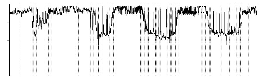
The first step to identify the average time of day at which these behavioral shifts occur was to use a split-moving window analysis (Ludwig and Cornelius 1987), which was applied to changes in time at depth. This approach has been used elsewhere to divide the vertical behaviour of free-roaming animals into behaviourally consistent sections over longer timescales (e.g., Humphries et al. 2010; Sims et al. 2011). Initially, the depth profiles for each individual were binned into proportion of time spent within 10-meter depth bins during each half-hour time period of the entire dive track. Then a ‘virtual’ window encompassing 24 time bins (12-hours) was placed at the start of the track, and split into two equal halves. Summing the proportion of time at each depth bin for each window half, the Euclidean distance was then calculated between the split-window. This is a measure of how dissimilar the first window half is from the second, in terms of time spent at different depths. This dissimilarity was recorded for the point in the binned depth profile split by the window, the window then moved on one bin, and the process was repeated for the new window position. In the case of tropical tuna, these measures of dissimilarity are often greatest when the window equally straddles a period of deeper behavior, typically during the day, and shallower behaviour, such as exhibited during the night, although this was not the case 100% of the time. There was also considerable inter-depth movement that did not correspond to these day/night periods. To identify when the most consistent shifts in movement occurred, the time at depth bins were shuffled 5000 times and the same analysis carried out. When these random dissimilarities failed to exceed those calculated from the originally ordered data at a particular point 95% of the time, we concluded that this represented a significant shift in vertical behaviour, given the variation in the data (Fig. A1).
Fig. A1. Example of ‘significant’ changes across a twelve-hour split moving window identified in an example section of dive track.
The periodicity of these significant behavioral changes was examined to identify whether there was a consistent, diel pattern in movement; significant changes can be expected to occur more commonly at the the day/night boundaries (crepuscular periods). A histogram of periods during the 24 hours in which significant changes occurred revealed the times at which those changes were most common. A K-means algorithm (MacQueen 1967; Hartigan and Wong 1979) was applied to estimate two clusters from the frequency of times of (a 24 hour) day at which significant changes occur. The center points of these clusters were selected as the crepuscular boundary periods that divide the dive data between day and night.
Once boundary periods had been identified, the data were further divided into the smaller units between the crepuscular boundary points. Summary metrics were calculated from the raw data for time bins of 1, 2, 3, 4, 6, 12 hours duration (an example is given in Fig. A2). At a time step of 3 hours, a balance was obtained between capturing dynamics such as just diving around crepuscular periods, or periods of ‘U-shaped’ diving, without the very fine patterns such as thermoregulatory dives being characterised individually in our analyses. Furthermore, such a time scale is appropriate for interpreting behavioral switching driven by underlying motivations that we believe are associated with feeding or digestion. For example, FAD-association is believed to occur on the scale of hours to months (Bromhead et al. 2003), whilst complete gastric evacuation occurs in tropical tuna at the scale of 5–12 hours (Olsen and Boggs 1986). We noted that at 12 and 6 hour time bins, the details of many shorter term and composite behaviors were also lost in the summary metrics, while noise from large individual dives began to increase at 2 and 1 hour sectioning. Summarising the dive data across three-hour sections provided variation across many different behavioral patterns, while retaining significant autocorrelation and smoothing some of the noise from those patterns unrelated to our study. Using this 3 hour interval as a guide we then subdivided each crepuscular period into four equally spaced time units. Although each section divided between dawn and dusk was equally spaced, depending on the time chosen for the crepuscular boundary, the day periods and night periods may not always contain exactly the same amount of data.
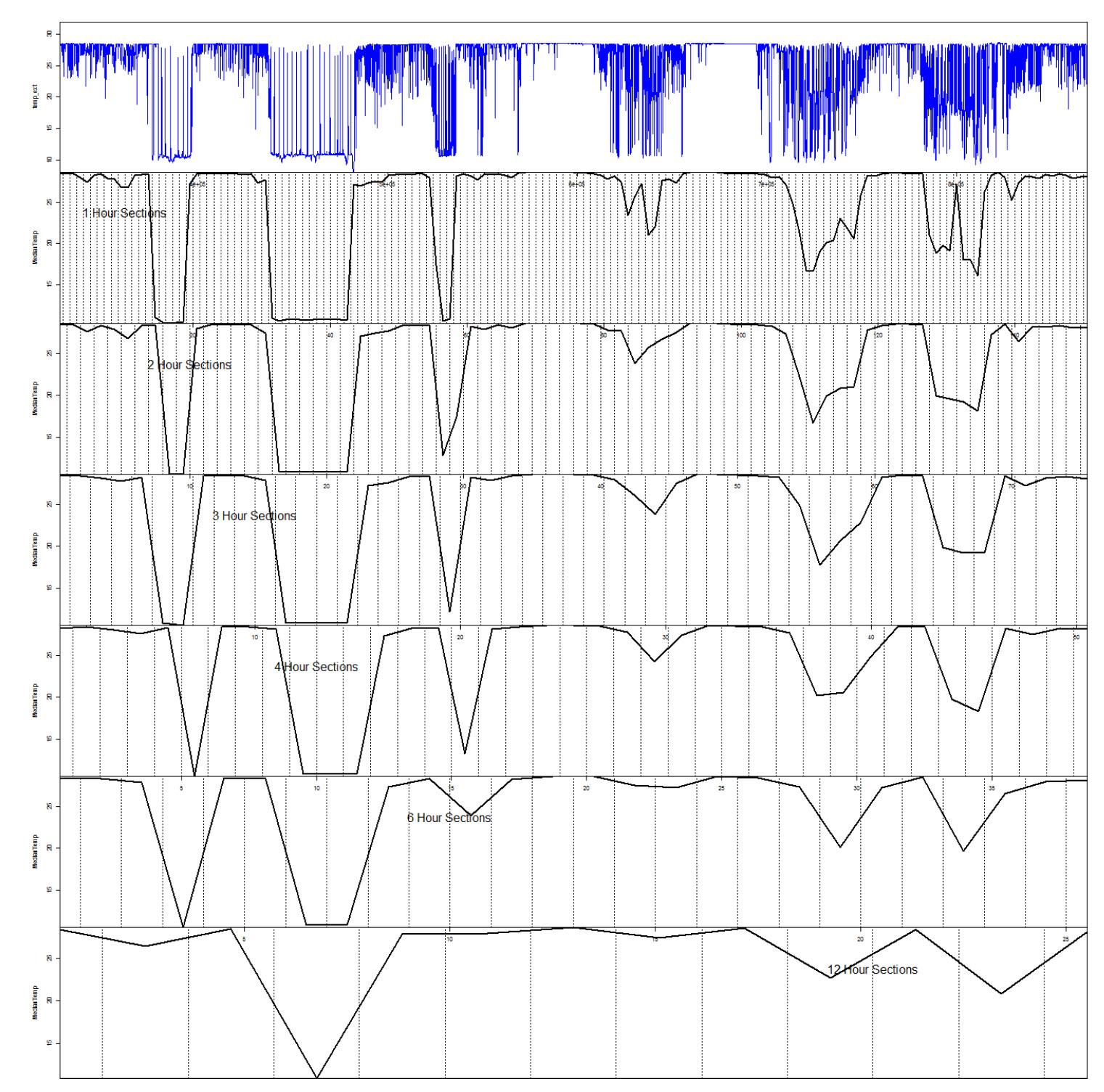
Fig. A2. Example of raw water temperature data processed into a summary metric of median temperature across increasing time bins.
In this study, we calculated an array of summary metrics from the available tag data across these time bins (pairwise examples from one individual are given in Fig. A3). As the study included tuna from different time periods and areas, we did not use measures of absolute depth which may differ across these factors for behaviors of the same underlying ecological motivation. We used a multivariate assemblage of summary metrics to capture information about both relative movement through the water column and temperature-based habitat use. Water temperature and absolute depth were highly correlated, although non-linearly. We used temperature as measure of habitat use. As individual deep and thermoregulatory dives can have a considerable effect on mean temperature metrics, the median water temperature was used. To choose the second summary metric in our multivariate assemblage, a principal component analysis was carried out on all the summary statistics (except absolute depth) calculated from individual fish to examine the ways in which the data may be transformed into orthogonal components. The standard deviation of depth provided consistently high loadings in the first principal component across a range of individual fish. We therefor chose this metric, a measure of vertical movement amplitude across the time bin, as the movement component of our multivariate normal observation model.
Thus, raw archival data was processed into a time-series containing a two-dimensional, multivariate assemblage of mean move step lengths and medium water temperatures across 3-hour time periods.
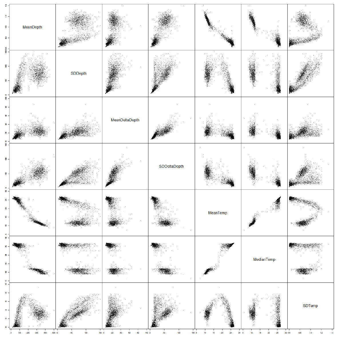
Fig. A3. Seven example summary metrics captured across three-hour time bins for a single time series, displayed as a grid of pairwise plots.
Literature cited
Bromhead, D., J. Foster, and R. Attard. 2003. A review of the impacts of fish aggregating devices (FADs) on tuna fisheries. Report to the Fisheries Resources Research Fund. BRS, Canberra.
Hartigan, J. A., and M. A. Wong. 1979. Algorithm AS 136: A k-means clustering algorithm. Journal of the Royal Statistical Society. Series C (Applied Statistics) 28(1):100–108.
Holan, S. H., G. Davis, M. L. Wildhaber, A. DeLonay, and D. Papoulias. 2009. Hierarchical Bayesian Markov Switching Models with Application to Predicting Spawning Success of Shovelnose Sturgeon. Journal of the Royal Statistical Society Series C. 58:47–64.
Humphries, N. E., N. Queiroz, J. R. M. Dyer,N. G. Pade, M. K. Musyl, K. M. Schaefer, D. W. Fuller, J. M. Brunnschweiler, T. K. Doyle, J. D. R. Houghton, G. C. Hays, C. S. Jones, L. R. Noble, V. J. Wearmouth, E. J. Southall, and D. W. Sims. 2010. Environmental context explains Lévy and Brownian movement patterns of marine predators. Nature 465:1066–9.
Ludwig, J. A., and J. M. Cornelius. 1987. Locating discontinuities along ecological gradients. Ecology 68:448–450.
Matsumoto, T., T. Kitagawa, and S. Kimura. 2013b. Vertical behavior of juvenile yellowfin tuna Thunnus albacares in the southwestern part of Japan based on archival tagging. Fisheries Science 79(3):417–424.
MacQueen, J. 1967. Some methods for classification and analysis of multivariate observations. In Proceedings of the fifth Berkeley symposium on mathematical statistics and probability (Vol. 1, p. 14).
Olson, R. J., and C. H. Boggs. 1986. Apex Predation by Yellowfïn Tuna (Thunnus albacares): Independent Estimates from Gastric Evacuation and Stomach Contents, Bioenergetics, and Cesium Concentrations. Canadian Journal of Fisheries and Aquatic Sciences 43(9):1760–1775.
Schaefer, K. M., and D. W. Fuller. 2004. Behavior of bigeye (Thunnus obesus) and skipjack (Katsuwonus pelamis) tunas within aggregations associated with floating objects in the equatorial eastern Pacific. Marine Biology 146(4):781–792.
Schaefer, K. M., D. W. Fuller, and B. A. Block. 2007. Movements, behavior, and habitat utilization of yellowfin tuna (Thunnus albacares) in the northeastern Pacific Ocean, ascertained through archival tag data. Marine Biology 152:503–525.
Sims, D. W., N. E. Humphries, R. W. Bradford, and B. D. Bruce. 2011. Lévy flight and Brownian search patterns of a free-ranging predator reflect different prey field characteristics. Journal of Animal Ecology:1–11.