Ecological Archives A025-059-A1

Christopher P. Kirol, Jeffrey L. Beck, Snehalata V. Huzurbazar, Matthew J. Holloran, and Scott N. Miller. 2015. Identifying Greater Sage-Grouse source and sink habitats for conservation planning in an energy development landscape. Ecological Applications 25:868–990. http://dx.doi.org/10.1890/13-1152.1

Appendix A. Additional survival and occurrence modeling results and individual resource selection functions and survival probability functions mapped on the landscape.

Table A1. Model category combinations (environmental and anthropogenic) considered in our sequential modeling approach predicting the relative probability of nesting sage-grouse occurrence in south-central Wyoming, USA, 2008 and 2009.

a Model categories (subsets) and associated predictor variables assessed individually and combined in our sequential modeling approach. Refer to Table 1 for predictor variable descriptions.

b Log-likelihood (LL), number of parameters (K), Akaike's Information Criterion adjusted for small sample sizes (AIC_c) score, change in AIC_c score from top model (ΔAIC_c), and Akaike weights (w_i).

Table A2. Model category combinations (environmental and anthropogenic) considered in our sequential modeling approach predicting the relative probability of female sage-grouse early brood-rearing occurrence in south-central Wyoming, USA, 2008 and 2009.

a Model categories (subsets) and associated predictor variables assessed individually and combined in our sequential modeling approach. Refer to Table 1 for predictor variable descriptions.
b Log-likelihood (LL), number of parameters (K), Akaike's Information Criterion adjusted for small sample sizes (AIC_c) score, change in AIC_c score from top model (ΔAIC_c), and Akaike weights (w_i).

Table A3. Model category combinations (environmental and anthropogenic) considered in our sequential modeling approach predicting the relative probability of non-brooding female sage-grouse occurrence during the early brood-rearing period in south-central Wyoming, USA, 2008 and 2009.

a Model categories (subsets) and associated predictor variables assessed individually and combined in our sequential modeling approach. Refer to Table 1 for predictor variable descriptions.
b Log-likelihood (LL), number of parameters (K), Akaike's Information Criterion adjusted for small sample sizes (AIC_c) score, change in AIC_c score from top model (ΔAIC_c), and Akaike weights (w_i).
c The true value is w_i = 0.999864.

Table A4. Model category combinations (environmental and anthropogenic) considered in our sequential modeling approach predicting the relative probability of female late brood-rearing occurrence in south-central Wyoming, USA, 2008 and 2009.

a Model categories (subsets) and associated predictor variables assessed individually and combined in our sequential modeling approach. Refer to Table 1 for predictor variable descriptions.
b Log-likelihood (LL), number of parameters (K), Akaike's Information Criterion adjusted for small sample sizes (AIC_c) score, change in AIC_c score from top model (ΔAIC_c), and Akaike weights (w_i).

Table A5. Model category combinations (environmental and anthropogenic) considered in our sequential modeling approach predicting the relative probability of non-brooding female occurrence during the late brood-rearing period in south-central Wyoming, USA, 2008 and 2009.

a Model categories (subsets) and associated predictor variables assessed individually and combined in our sequential modeling approach. Refer to Table 1 for predictor variable descriptions.
b Log-likelihood (LL), number of parameters (K), Akaike's Information Criterion adjusted for small sample sizes (AIC_c) score, change in AIC_c score from top model (ΔAIC_c), and Akaike weights (w_i).

Table A6. Model category combinations (environmental and anthropogenic) considered in our sequential modeling approach predicting brood survival to 36 days in south-central Wyoming, USA, 2008 and 2009.

a Model categories (subsets) and associated predictor variables assessed individually and combined in our sequential modeling approach. Refer to Table 1 for predictor variable descriptions.
b Log-likelihood (LL), number of parameters (K), Akaike's Information Criterion adapted for survival models (AICSUR) score, change in AICSUR score from top model (ΔAICSUR), and Akaike weights (w_i).

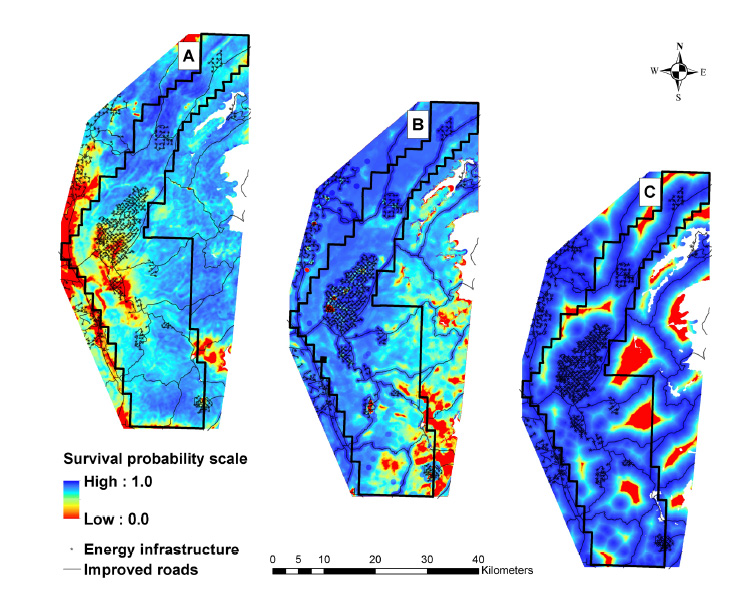
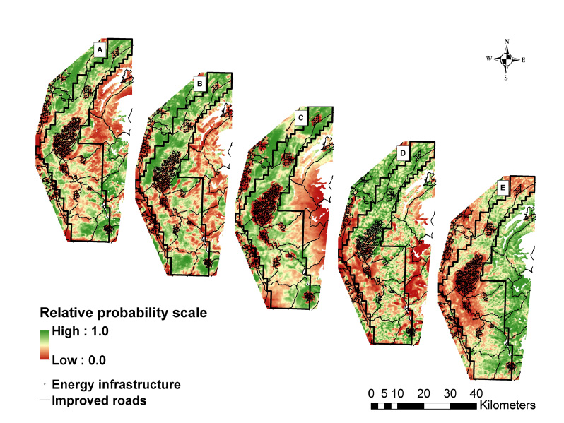
Fig. A1. Relative probability of (A) nesting, (B) early brood-rearing, (C) early non-brooding, (D) late brood-rearing, and (E) late non-brooding sage-grouse occurrence in south-central, Wyoming, USA, 2008 and 2009. These predictive maps are model averaged resource selection functions with 1 (green) being the highest and 0 (red) being the lowest probability of occurrence. The maps were weighted based on the importance to λ, overlaid, and summed to form the female sage-grouse summer occurrence map (Fig. 2).

Fig. A2. Relative probability of sage-grouse (A) nest survival to 28 days, (B) brood survival to 36 days, and (C) adult female survival to 110 days. Mapped as a survival probability function in south-central, Wyoming, USA, 2008 and 2009. The maps predict the probability of survival with 1 (blue) being the highest and 0 (red) being the lowest probability. When interpreting the survival maps one should consider that, in some instances, the predictive surface may be predicting survival in habitats with low sage-grouse occurrence (see Fig. 5) thus the survival maps should be considered in context of habitat use (Fig. A1).

[Back to A025-059]