Ecological Archives A025-039-A2
Brian D. Gerber and Robert P. Parmenter. 2015. Spatial capturerecapture model performance with known small-mammal densities. Ecological Applications 25:695705. http://dx.doi.org/10.1890/14-0960.1
Appendix B. Point and interval estimates of abundance and density of small-mammal populations, the fully specified Bayesian Null SCR model, the demonstration of a skewed posterior distribution on measures of central tendency and measures of uncertainty, and linear regression analyses of ![]() vs. D.
vs. D.
Table B1. Small-mammal density (![]() ,individuals / ha) and abundance estimates (
,individuals / ha) and abundance estimates (![]() ) of populations sampled using a trapping web. A null spatial-capture recapture model (SCR) was fitted using a maximum likelihood (ML) and Bayesian approach. Bayesian point estimate is the posterior mode and uncertainty is expressed as 95 % lower and upper confidence (CI) and highest posterior density (HPD) intervals.
) of populations sampled using a trapping web. A null spatial-capture recapture model (SCR) was fitted using a maximum likelihood (ML) and Bayesian approach. Bayesian point estimate is the posterior mode and uncertainty is expressed as 95 % lower and upper confidence (CI) and highest posterior density (HPD) intervals.
Population Number by Species |
True Abundance / |
ML SCR |
ML SCR |
Bayesian SCR |
Bayesian SCR |
|
Perognathus flavus |
||||||
1 |
88 / 20.57 |
18.22 (12.42 – 26.72) |
77.53 (52.72 – 113.39) |
17.52 (11.91 – 26.86) |
75 (51 – 115) |
|
2a |
39 / 9.44 |
NA |
NA |
NA |
NA |
|
3 |
58 / 13.83 |
15.21 (11.18 – 20.68) |
63.55 (54.02 – 78.14) |
14.29 (11.43 – 20.96) |
60 (45 – 85) |
|
4 |
81 / 19.06 |
17.10 (12.64 – 23.12) |
72.82 (61.30 – 90.57) |
16.70 (12.47 – 23.05) |
71 (53 – 98) |
|
Cricetines |
||||||
5 |
65 / 15.73 |
12.72 (11.93 – 13.56) |
53.42 (49.64 – 56.42) |
12.59 (12.34 – 13.55) |
52 (51 – 56) |
|
6 |
22 / 5.24 |
3.74 (3.38 – 4.12) |
15.56 (14.06 – 17.21) |
3.57 (3.57 – 4.05) |
15 (15 – 17) |
|
7 |
33 / 7.76 |
4.87 (3.71 – 6.38) |
21.06 (15.76 – 27.06) |
4.70 (4.00 – 6.35) |
20 (17 – 27) |
|
8 |
33 / 7.71 |
6.87 (6.22 – 7.60) |
29.66 (26.38 – 32.24) |
6.77 (6.54 – 7.48) |
29 (28 – 32) |
|
Peromyscus maniculatu |
||||||
9 |
26 / 6.29 |
5.78 (5.15 – 6.50) |
24.56 (21.41 – 27.04) |
5.81 (5.57 – 6.53) |
24 (23 – 27) |
|
10 |
14 / 3.27 |
2.45 (1.68 – 3.57) |
10.83 (7.14 – 15.14) |
2.34 (2.1 – 3.74) |
10 (9 – 16) |
|
Dipodomys spp. |
||||||
11 |
18 / 4.29 |
3.89 (2.69 – 5.63) |
16.55 (11.18 – 23.43) |
3.57 (2.86 – 5.24) |
15 (12 – 22) |
|
a No individuals were recaptured at more than one trap, precluding SCR model estimation
Table B2. Small-mammal density (![]() ,individuals / ha) and abundance estimates (
,individuals / ha) and abundance estimates (![]() ) of populations sampled using a trapping web. A spatial-capture recapture model (SCR) with a behavioral effect was fitted using a maximum likelihood (ML) and Bayesian approach. Bayesian point estimate is the posterior mode and uncertainty is expressed as 95 % lower and upper confidence (CI) and highest posterior density (HPD) intervals.
) of populations sampled using a trapping web. A spatial-capture recapture model (SCR) with a behavioral effect was fitted using a maximum likelihood (ML) and Bayesian approach. Bayesian point estimate is the posterior mode and uncertainty is expressed as 95 % lower and upper confidence (CI) and highest posterior density (HPD) intervals.
Population Number by Species |
True Abundance / |
ML-SCR |
ML-SCR |
Bayesian SCR |
Bayesian SCR |
||
Perognathus flavus |
|||||||
1 |
88 / 20.57 |
10.87 (8.42 – 14.04) |
46.49 (35.72 – 59.56) |
10.51 (8.41 – 15.18) |
45 (36 – 65) |
||
2 |
39 / 9.44 |
NA |
NA |
NA |
NA |
||
3 |
58 / 13.83 |
13.56 (9.55 – 19.25) |
56.75 (39.75 – 80.12) |
12.62 (9.77 – 22.63) |
53 (39 – 93) |
||
4 |
81 / 19.06 |
20.39 (11.81 – 35.20) |
86.76 (50.12 – 149.37) |
19.76 (12.47 – 41.63) |
84 (53 – 177) |
||
Cricetines |
|||||||
5 |
65 / 15.73 |
12.49 (11.83 – 13.18) |
52.48 (49.24 – 54.84) |
12.34 (12.34 – 13.31) |
51 (51 – 55) |
||
6 |
22 / 5.24 |
3.78 (2.27 – 6.30) |
15.73 (13.82 – 17.90) |
3.57 (3.57 – 4.53) |
15 (15 – 19) |
||
7 |
33 / 7.76 |
4.90 (3.51 – 6.38) |
21.19 (14.90 – 28.99) |
4.70 (4.00 – 10.82) |
20 (17 – 46) |
||
8 |
33 / 7.71 |
6.70 (6.17 – 7.27) |
28.96 (26.20 – 30.87) |
6.54 (6.54 – 7.48) |
28 (28 – 32) |
||
Peromyscus maniculatu |
|||||||
9 |
26 / 6.29 |
5.55 (5.11 – 6.03) |
23.65 (21.28 – 25.08) |
5.57 (5.57 – 6.05) |
23 (23 – 25) |
||
10 |
14 / 3.27 |
2.34 (1.57 – 3.48) |
10.37 (6.66 – 14.76) |
2.10 (2.10 – 7.71) |
9 (9 – 33) |
||
Dipodomys spp. |
|||||||
11 |
18 / 4.29 |
4.21 (2.35 – 7.55) |
17.85 (9.76 – 31.41) |
3.81 (2.86 – 0.24) |
16 (12 – 43) |
||
Table B3. Small-mammal density (![]() ,individuals / ha) and abundance estimates (
,individuals / ha) and abundance estimates (![]() ) of populations sampled using a trapping grid. A null spatial-capture recapture model (SCR) was fitted using a maximum likelihood (ML) and Bayesian approach. Bayesian point estimate is the posterior mode and uncertainty is expressed as 95 % lower and upper confidence (CI) and highest posterior density (HPD) intervals.
) of populations sampled using a trapping grid. A null spatial-capture recapture model (SCR) was fitted using a maximum likelihood (ML) and Bayesian approach. Bayesian point estimate is the posterior mode and uncertainty is expressed as 95 % lower and upper confidence (CI) and highest posterior density (HPD) intervals.
Population Number by Species |
True Abundance / |
ML-SCR |
ML-SCR |
Bayesian SCR |
Bayesian SCR |
||
Perognathus flavus |
|||||||
1 |
88 / 20.57 |
33.77 (24.22 – 47.09) |
143.49 (102.79 – 199.85) |
31.30 (23.36 – 46.95) |
134 (98 – 199) |
||
2 |
39 / 9.44 |
3.55 (1.45 – 8.70) |
14.92 (6.01 – 36.21) |
2.90 (1.21 – 11.62) |
12 (5 – 48) |
||
3 |
58 / 13.83 |
15.62 (11.10 – 21.99) |
65.23 (46.20 – 91.52) |
14.29 (10.24 – 20.96) |
60 (43 – 88) |
||
4 |
81 / 19.06 |
28.46 (19.39 – 41.76) |
120.93 (82.28 – 177.22) |
26.11 (17.40 – 40.22) |
111 (74 – 171) |
||
Cricetines |
|||||||
5 |
65 / 15.73 |
11.78 (9.68 – 14.33) |
49.40 (40.28 – 59.63) |
11.13 (9.68 – 13.55) |
46 (40 – 56) |
||
6 |
22 / 5.24 |
4.89 (3.89 – 6.16) |
20.81 (16.17 – 25.65) |
4.53 (4.29 – 5.95) |
19 (18 – 25) |
||
7 |
33 / 7.76 |
5.77 (4.40 – 7.57) |
24.90 (18.68 – 32.12) |
5.41 (4.70 – 7.53) |
23 (20 – 32) |
||
8 |
33 / 7.71 |
6.56 (5.39 – 7.98) |
28.28 (22.89 – 33.88) |
5.84 (5.61 – 7.24) |
25 (24 – 31) |
||
Peromyscus maniculatu |
|||||||
9 |
26 / 6.29 |
4.18 (3.17 - 5.51) |
17.82 (13.19 – 22.91) |
4.11 (3.63 – 5.57) |
17 (15 – 23) |
||
10 |
14 / 3.27 |
3.54 (2.59 - 4.84) |
15.46 (11.00 – 20.53) |
3.27 (3.04 – 4.91) |
14 (13 – 21) |
||
Dipodomys spp. |
|||||||
11 |
18 / 4.29 |
4.37 (2.86 – 6.72) |
18.64 (11.89 – 27.96) |
3.81 (3.57 – 5.72) |
16 (15 – 24) |
||
Table B4. Small-mammal density (![]() ,individuals / ha) and abundance estimates (
,individuals / ha) and abundance estimates (![]() ) of populations sampled using a trapping grid. A spatial-capture recapture model (SCR) with a behavioral effect was fitted using a maximum likelihood (ML) and Bayesian approach. Bayesian point estimate is the posterior mode and uncertainty is expressed as 95 % lower and upper confidence (CI) and highest posterior density (HPD) intervals.
) of populations sampled using a trapping grid. A spatial-capture recapture model (SCR) with a behavioral effect was fitted using a maximum likelihood (ML) and Bayesian approach. Bayesian point estimate is the posterior mode and uncertainty is expressed as 95 % lower and upper confidence (CI) and highest posterior density (HPD) intervals.
Population Number by Species |
True Abundance / |
ML-SCR |
ML-SCR |
Bayesian SCR |
Bayesian SCR |
|
Perognathus flavus |
||||||
1 |
88 / 20.57 |
27.38 (19.67 – 38.1) |
116.38 (83.48 – 161.66) |
25.23 (17.99 – 46.49) |
108 (75 – 197) |
|
2 |
39 / 9.44 |
2.18 (1.03 – 4.61) |
9.33 (4.28 – 19.18) |
1.21 (1.21 – 3.63) |
5 (5 – 15) |
|
3 |
58 / 13.83 |
14.52 (10.03 – 21.02) |
60.64 (41.73 – 87.47) |
14.05 (8.57 – 25.49) |
59 (36 – 107) |
|
4 |
81 / 19.06 |
19.19 (13.51 – 27.26) |
81.69 (57.31 – 115.69) |
17.64 (11.76 – 28.93) |
75 (50 – 123) |
|
Cricetines |
||||||
5 |
65 / 15.73 |
13.71 (9.99 – 18.82) |
57.4 (41.57 – 78.32) |
13.31 (9.92 – 22.99) |
55 (41 – 95) |
|
6 |
22 / 5.24 |
6.46 (3.59 – 11.61) |
27.2 (14.94 – 48.33) |
4.53 (4.29 – 5.95) |
19 (18 – 25) |
|
7 |
33 / 7.76 |
4.79 (4.26 – 5.38) |
20.85 (18.08 – 22.84) |
4.70 (4.70 – 5.64) |
20 (20 – 24) |
|
8 |
33 / 7.71 |
6.03 (5.14 – 7.07) |
26.07 (21.82 – 30.02) |
5.84 (5.61 – 6.77) |
25 (24 – 29) |
|
Peromyscus maniculatu |
||||||
9 |
26 / 6.29 |
4.61 (2.99 – 7.11) |
19.56 (12.42 – 29.58) |
4.60 (3.63 – 10.41) |
19 (15 – 43) |
|
10 |
14 / 3.27 |
3.23 (2.76 – 3.79) |
13.72 (11.71 – 16.09) |
3.04 (3.04 – 3.97) |
13 (13 – 17) |
|
Dipodomys spp. |
||||||
11 |
18 / 4.29 |
3.83 (3.17 – 4.63) |
15.95 (13.21 – 19.26) |
3.57 (3.57 – 5.00) |
15 (15 – 21) |
|
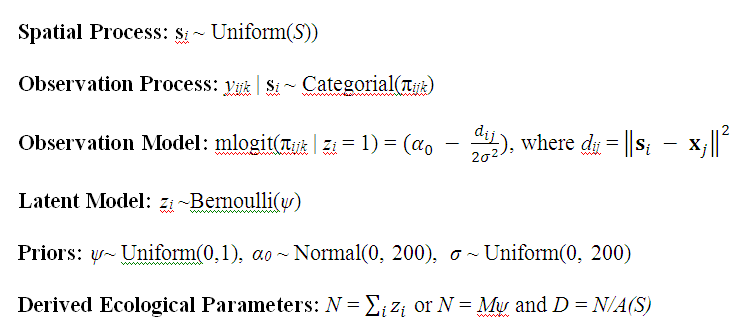
Fig. B1. The Null Bayesian hierarchical spatial capture–recapture model, specified for an augmented capture-history. Indexing is by individual i = 1, 2, … , M, trap j = 1, 2, …, J, and sample interval (occasion) k = 1, 2, … , K. x is a J × 2 matrix of trap coordinates, s is a matrix of activity center coordinates, where si = sxi, syi, and A(S) is the area of the state-space, S.
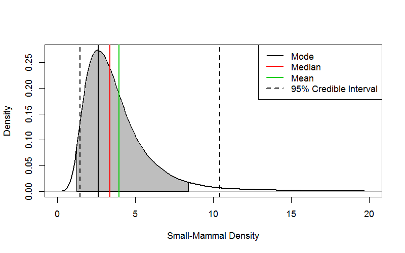
Fig. B2. The posterior distribution of small-mammal density of population 2 sampled using a trapping grid and analyzed with the Null spatial capture–recapture model. The positively skewed posterior distribution clarifies difference among measures of central tendency and between the
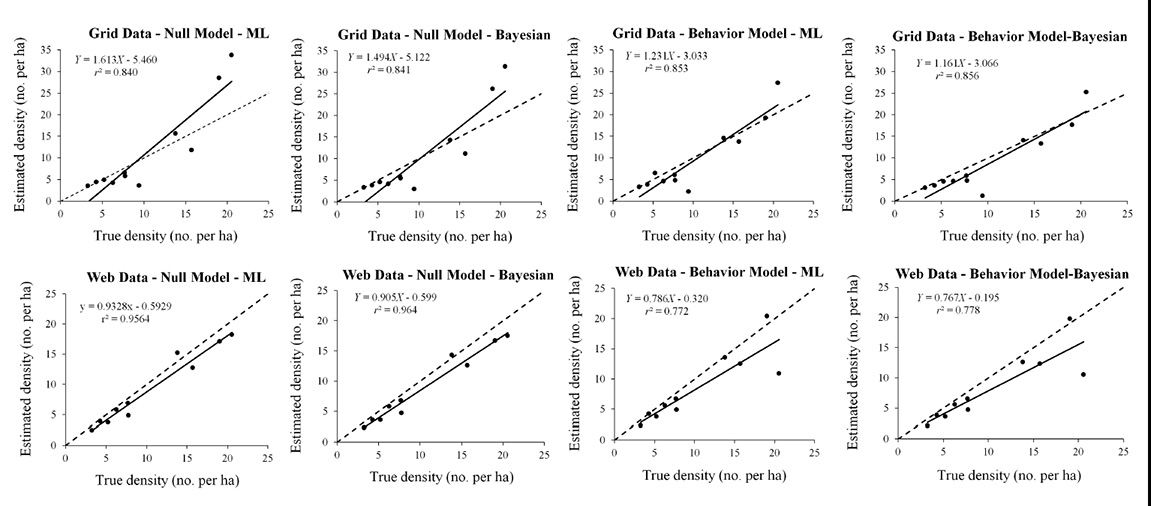
Fig. B3. Linear regression test of the accuracy of spatial-capture recapture models. Dashed diagonal line indicates equality between true density and density estimates. More accurate estimators have a slope closer to 1 and a higher coefficient of determination r².