![]()
Ecological Archives A025-034-A5
Jeffrey F. Bromaghin, Trent L. McDonald, Ian Stirling, Andrew E. Derocher, Evan S. Richardson, Eric V. Regehr, David C. Douglas, George M. Durner, Todd Atwood, and Steven C. Amstrup. 2015. Polar bear population dynamics in the southern Beaufort Sea during a period of sea ice decline. Ecological Applications 25:634651. http://dx.doi.org/10.1890/14-1129.1
Appendix E. Projected trends in the abundance of southern Beaufort Sea polar bears based on estimated survival rates.
Capture probabilities ofsouthern Beaufort Sea polar bears are thought to vary primarily in response to environmental and ecological conditions that influence their movements and spatial distribution. Unfortunately, our ability to identify and measure pertinent variables and incorporate them into models as covariates is limited. Because abundance estimates in Cormack-Jolly-Seber (CJS) models are derived from estimated recapture probabilities using the Horvitz-Thompson (HT) estimator (McDonald and Amstrup 2001), un-modeled structure in recapture probabilities has the potential to introduce bias. As noted in the summary of USGS modeling results, estimates in the first two years, particularly 2002, are suspected of being negatively biased by the absence of capture effort from Barrow in 2001, the incomplete accumulation of marked individuals in the population (Appendix B, Table B1), and perhaps non-random movement between consecutive years (Appendix D, Fig. D2). In addition, the unusually large number of bears captured in 2004 (Table 5) may be responsible for the seemingly large point estimate of abundance in that year (Fig. 5). With respect to the USCA estimates, a lack of Canadian capture effort before 2003, as well as reduced effort and lack of capture effort in the easternmost portion of the study area after 2006, may have introduced bias into those abundance estimates, despite our attempts to model known factors potentially influencing recapture probabilities.
To investigate whether potential biases in abundance estimates might have influenced the assessment of abundance status and trend, we conducted simulations to project abundance from 2001 to 2010 based only on estimated survival probabilities, which are more robust to un-modeled heterogeneity in recapture probabilities that can bias abundance estimates (Carothers 1979, Abadi et al. 2013). USGS capture data from 1989 to 2003 were pooled and used to develop an initial probability distribution f of bears among sex, age, and family categories. Captured individuals were jointly classified by sex and age, and family groups were classified by the number and age of dependent young. The maximum age observed from 1989 to 2003 was 29, which was utilized as the maximum possible age in the simulations. The number of observations in each of the resulting 206 combinations of sex, age, and family categories was counted, and each count was increased by one so that all categories had a nonzero probability of occurring. The counts were additionally adjusted to account for the 2002–2010 mean model-averaged estimate of recapture probability for each category (Appendix C), and the resulting values were scaled to sum to 1.0 to constitute a probability distribution f for the demographic composition of the population in the initial year of 2001. The 1989–2003 USGS capture data were similarly used to construct a probability distribution g for the number of cubs in a family group (1, 2, or 3).
Initial populations of USGS and USCA bears were randomly established in 2001. Because the USGS abundance estimate from 2002, and possibly the estimates from 2003 and 2004, was suspected of being biased, as noted above, the mean initial population size was established at 1,000 individuals, the approximate mean of the 2003 and 2004 estimates. A mean initial abundance of 1,500 bears was used for the USCA population, which was approximately equal to the mean abundance estimate of 1,526 for the period 2004–2006 reported by Regehr et al. (2006). Note that these starting points are not consequential, as the trend in relative abundance through time is of primary interest. In each case, the initial population size was divided by the mean number of individuals per category in the probability distribution f to derive a sample size, accounting for multiple individuals in family groups which were sampled as a unit, and a multinomial sample of the resulting size was drawn from f to establish initial populations in 2001.
The initial populations randomly established in 2001 were projected forward in time to 2010 using survival rates. The estimated survival probabilities obtained by bootstrapping were first bias-corrected so that their means equaled the point estimates of survival (Figs. 3 and 4). In each year, a mean annual survival probability for each sex and age class was randomly drawn from the bias-corrected bootstrap estimates. Given the resulting survival probability for each sex and age class, survival was established by drawing a random Bernoulli deviate for each individual in the population. All individuals that survived to the maximum age of 29 died prior to the following year. If an adult female with dependent young died, the young also died. If a female survived but all her dependent young died, she was available to reproduce the following year.
A measure of production (B) related to the litter production rate (Ramsay and Stirling 1988) and breeding success (Wiig 1998)
was computed from the spring capture data each year from 2002 to 2010 and used to established new litters for a portion of the females without dependent young. Although B does not incorporate mortality over the interval from birth to the capture of a female with cubs, that is consistent with CJS estimates of cub survival. Given the value of B in any one year, a random Bernoulli deviate was drawn to determine if each adult female without dependent young acquired a new litter of cubs. Litter sizes for reproductive females were randomly established using the probability distribution g. Consistent with the structure of the mark-recapture models used in the analysis, the sex of yearlings that survived to age 2, the youngest sub-adult age, was established with a random Bernoulli deviate having a mean of 0.5.
The sequence of randomly establishing an initial population in 2001 and projecting abundance forward in time to 2010 by simulating survival and births was replicated 1,000 times; simulations for the USGS and USCA data sets were independent. The mean abundance across replications in each year was plotted along with the 5th and 95th quantiles as error bars (Figs. E1 and E2). Mean projected abundance across replications in each year was scaled to minimize the squared difference between the mean projection and estimated abundance, weighted by the inverse width of abundance confidence intervals, and plotted with point estimates of abundance and their 90% confidence intervals to facilitate a comparison of their trends (Fig. E3, E4).
Trends in abundance from the projections were similar to the trends in the abundance estimates, excepting the earliest years in which the estimates are suspected of being biased. The projected abundance trends with both data sets increased through 2004 and declined through 2007 (Figs. E1 and E2). The rate of decline in USGS projections moderated from 2009 to 2010 and the USCA projections were stable from 2008 to 2010. The correlation between the estimated and projected USGS abundance trends from 2002 to 2010 was 0.85, and 0.90 from 2003 to 2010 (Fig. E3). The corresponding correlations for the USCA trends were 0.89 from 2002 to 2010 and 0.95 from 2003 to 2010 (Fig. E4).
Given that the abundance projections are partially independent of the abundance estimates, their concordance increases confidence in our finding that a period of low survival from 2004 to 2006 led to a substantial decline in the abundance of polar bears in the southern Beaufort Sea.
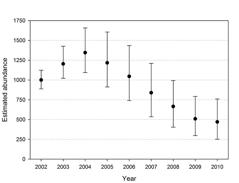
Fig. E1. Abundance trends of southern Beaufort Sea polar bears observed across replications of the population projection based on survival rates estimated with the USGS data set. Error bars denote the 5th and 95th quantiles observed across the 1,000 replications.
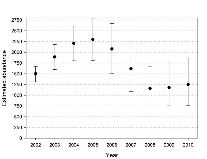
Fig. E2. Abundance trends of southern Beaufort Sea polar bears observed across replications of the population projection based on survival rates estimated with the USCA data set. Error bars denote the 5th and 95th quantiles observed across the 1,000 replications.
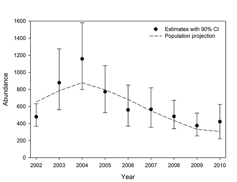
Fig. E3. Annual abundance estimates with 90% bias-corrected bootstrap confidence intervals for southern Beaufort Sea polar bears based on the USGS data set, and the re-scaled mean annual abundance observed during the 1,000 replications of the USGS population projection.
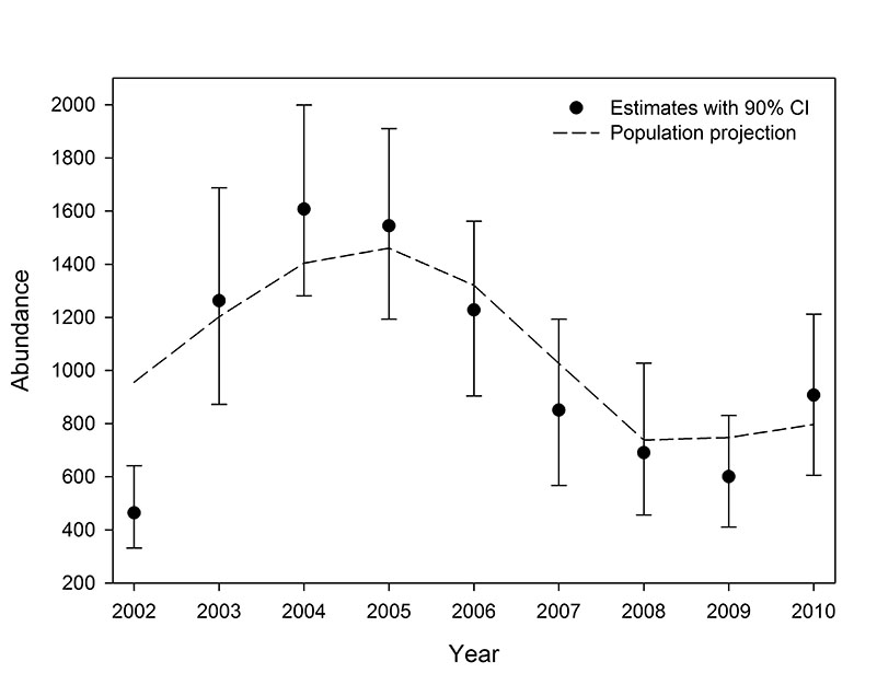
Fig. E4. Annual abundance estimates with 90% bias-corrected bootstrap confidence intervals for southern Beaufort Sea polar bears based on the USCA data set, and the re-scaled mean annual abundance observed during the 1,000 replications of the USCA population projection.
Literature cited
Abadi, F., A. Botha, and R. Altwegg. 2013. Revisiting the effect of capture heterogeneity on survival estimates in capture-mark-recapture studies: Does it matter? PLoS One 8:e62636.
Carothers, A. D. 1979. Quantifying unequal catchability and its effect on survival estimates in an actual population. Journal of Animal Ecology 48:863–869.
McDonald, T. L., and S. C. Amstrup. 2001. Estimation of population size using open capture–recapture models. Journal of Agricultural, Biological, and Environmental Statistics 6:206–220.
Ramsay, M. A., and I. Stirling. 1988. Reproductive biology and ecology of female polar bears (Ursus maritimus). Journal of Zoology 214:601–634.
Regehr, E. V., S. C. Amstrup, and I. Stirling. 2006. Polar bear population status in the southern Beaufort Sea: U.S. Geological Survey Open-File Report 2006–1337.
Wiig, Ø. 1998. Survival and reproductive rates for polar ears at Svalbard. Ursus 10:25–32.