Ecological Archives A025-016-A2

Ryan McManamay and Emmanuel A. Frimpong. 2015. Hydrologic filtering of fish life history strategies across the United States: implications for stream flow alteration. Ecological Applications 25:243–263. http://dx.doi.org/10.1890/14-0247.1

Appendix B. Justification for inclusion and methods for summarizing landscape variables for use in predicting fish traits, summary of correlations among predictors and trait-frequencies, and an assessment of redundancy in predictors.

1. Landscape Variables: Justification and Summarization Methods

Geology

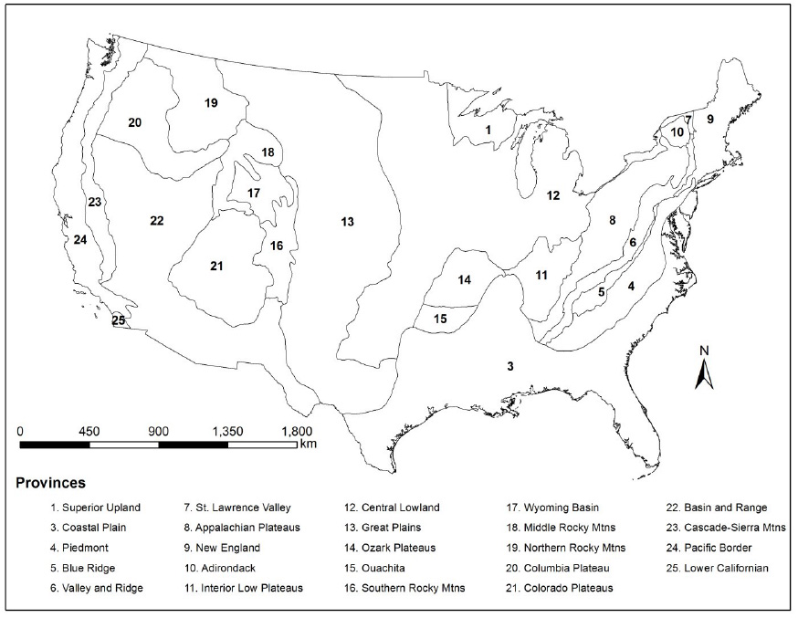
Geology exerts strong influences on fish assemblage structure because the underlying lithology determines the buffering capacity and morphological complexity of aquatic habitats (Jackson and Harvey 1989). Geology was represented by three variables: physiographic provinces, percent sand, and bedrock permeability. Physiographic provinces represent areas of similar topography, rock types, and geologic/geomorphic history (Fenneman and Johnson 1946, Fig. B1). Physiographic provinces provide suitable boundaries to stratify stream channel morphology relationships (Johnson and Fecko 2008) and areas of distinct water chemistry (Lowrance et al. 1997; Apodaca and Bails 2000; Swain et al. 2004). Percent sand and bedcrock permeability classes both provide a measure of geologic texture (Wolock et al. 2004), but are also an indication of different lithology-related influences on water physiochemistry (Lindsey et al. 2009). Bedrock permeability represents different aquifer types and ranges from 1 to 7, with 7 having the highest permeability (Wolock et al. 2004). Using intersection methods, the dominant physiographic province was summarized within all HUC8 subbasins. Percent sand and bedrock permeability were available as summaries within small catchments (Wolock et al. 2004), which we aggregated and averaged to the larger HUC8 subbasins.

Topography

Topography, similar to geology, exerts controls on aquatic habitat structure (Jackson et al. 2001). We compiled elevation, relief, slope, and % flat land to describe variation in topography. Elevation was available as a 1-km grid raster for the U.S. (Hastings et al. 1999). We used zonal statistics (Spatial Analyst Tools) to calculate the mean, minimum, and maximum elevation within each HUC8. Relief was calculated as the difference in maximum and minimum elevation. Slope (% rise) and % flat land (% of area with slopes < 1%) were available as summaries within small catchments (Wolock et al. 2004) and were aggregated and averaged to HUC8 subbasins.

Climate

Climate variables, especially precipitation, could be viewed as redundant if used in combination with hydrologic variables. However, precipitation may provide gross regional differences not captured in hydrologic metrics. Precipitation and temperature as 30-year averages (1981-2010) were available as 1-km² grids across the U.S. (PRISM 2013). Using zonal statistics, we calculated the mean, minimum, and maximum elevation with each HUC8. Potential evapotranspiration and water stress (precipitation – potential evapotranspiration) were summarized within small catchments (Wolock et al. 2004), which were aggregated to HUC8 subbasin.

Fig. B1. Physiographic provinces of the conterminous US.

Landcover

Landcover types were included as additional variables to aid in discriminating amongst adjacent watersheds, since the presence of fish species may depend on local vegetation, wetlands, or land use. We accessed the 2001 National Land Cover Database, rather than the 2006 version, because the temporal extent of 2001 data overlapped more accurately with the origination of fish assemblage data (NatureServe 2004). High collinearity among land cover types can lead to spurious conclusions of the importance of landcover on ecological patterns (King et al. 2005); thus, because of the predominance of forest vegetation and high correlation with other land cover types, we excluded forest land cover categories with preference for less common land cover types. Because fish assemblage lists were historically comprehensive for watersheds (NatureServe 2004), the primary focus was on natural rather than anthropogenic landscape patterns. However, landscape disturbances, such as agriculture and development, may predate even historical accounts of fish species presence and thus, leave legacy impacts on species distribution. We combined all developed, agriculture, and wetland coverages into composite land cover types for each respective category. Open water cover, ice and snow, barren lands, scrubland, and herbaceous land cover represented individual variables important to fish assemblages. We used zonal statistics to summarize the percent area of land cover types within each HUC8 subbasin.

Ecosystem Productivity

Ecosystem productivity has been shown to be positively related with fish diversity (Guégan et al. 1998) and an important predictor of fish life history strategies (Olden and Kennard 2010). Net terrestrial primary productivity (NPP) was included to account for available energy. We obtained NPP (metric tons of carbon km^-2) as a raster grid data set (Imholf et al. 2004) and calculated mean NPP for each HUC-8 using zonal statistics.

2. Correlations among predictor and response variables:

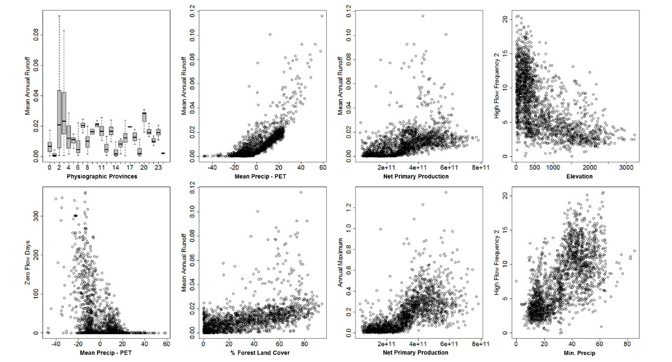
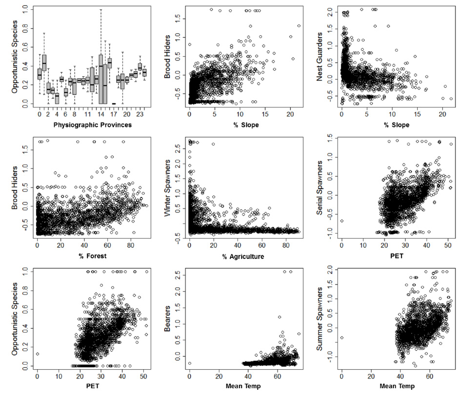
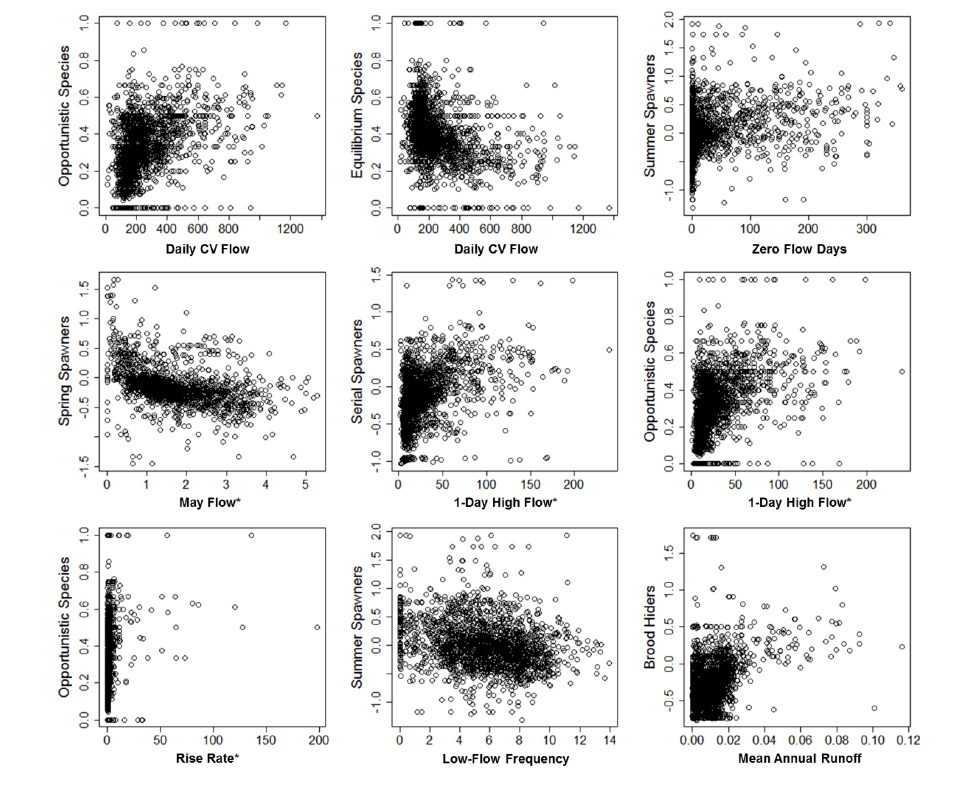
Correlations among predictor variables, and between predictor variables and trait frequencies were explored using Spearman's rank correlations. Examples of stronger correlations are provided in Figs. B1–B3. A correlation matrix of pair-wise comparisons of trait-by-trait frequencies is provided in Table B1.

3. Partial variance and overlap in predictor variables:

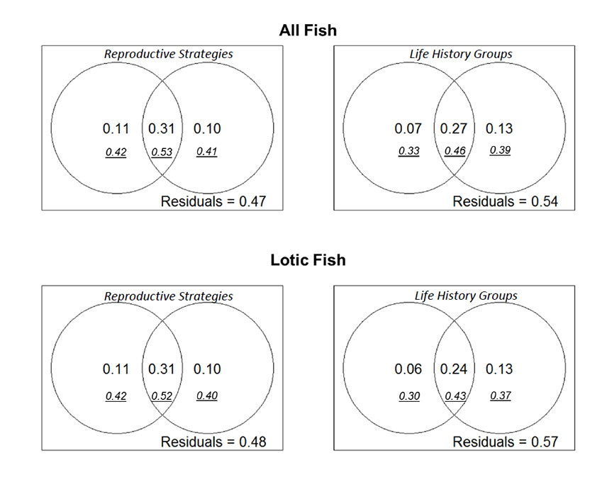
To determine the relative contribution of hydrology in explaining fish trait frequencies, we used redundancy analysis (RDA) to examine partial variation between hydrology, landscape variables, and their combined effect. Partial variance was calculated for hydrology and landscape variables. Venn diagrams were used to represent the partial variance fractions and overlapping variance between hydrologic and landscape predictors (Fig. B4).

Fig. B2. Examples of correlations among landscape and hydrologic predictor variables

Fig. B3. Examples of correlations among landscape variables and fish trait frequencies

Fig. B4. Examples of correlations among hydrologic variables and fish trait frequencies

Table B1. Spearman's rank correlation matrix of pairwise comparisons of trait-frequencies summarized within HUC-8 subbasins. Values > or < 0.6 are in bold.

Fig. B5. Venn diagrams representing partial variance fractions and overlapping variance between hydrologic and landscape predictors in explaining fish trait frequencies. Larger numbers represent partial fractions (hydrology on left, landscape on right) whereas underlined smaller numbers represent total % variance. Fish trait frequencies were broken into two groups (reproductive strategies and life history groups) and were separately analyzed for all fish and then, only lotic fish.

Literature cited

Apodaca, L. E., and J. B. Bails. 2000. Water quality in alluvial aquifers of the Southern Rocky Mountains Physiographic Province, Upper Colorado River Basin, Colorado, 1997. U.S. Geological Survey Water-Resources Investigations Report 99 –4222. Denver, CO. 68pp.

Fenneman, N. M., and D. W. Johnson. 1946. Physiographic Divisions of the Conterminous US: U.S. Geological Survey Special Map Series, Scale 1:7,000,000 , Reston, VA. Available at: http://water.usgs.gov/GIS/metadata/usgswrd/XML/physio.xml

Guégan, J. F., S. Lek, and T. Oberdorff. 1998. Energy availability and habitat heterogeneity predict global riverine fish diversity. Nature 391: 382-384.

Hastings, D. A., P. K. Dunbar, G. M. Elphingstone, M. Bootz, H. Murakami, H. Maruyama, H.Masaharu, P. Holland, J. Payne, N. A. Bryant, T. L. Logan, J. -P. Muller, G. Schreier, and J. S. MacDonald. 1999. The Global Land One-kilometer Base Elevation (GLOBE) digital elevation model, Version 1.0. National Oceanic and Atmospheric Administration, National Geophysical Data Center. Accessed July 9, 2013 at: http://www.ngdc.noaa.gov/mgg/topo/globe.html .

Imhoff, M. L., L. Bounoua, T. Ricketts, C. Loucks, R. Harriss, and W. T. Lawrence. 2004. Global Patterns in Net Primary Productivity. Socioeconomic Data and Applications Center (SEDAC). Accessed September 12, 2012 at: http://sedac.ciesin.columbia.edu/es/hanpp.html.

Jackson, D.A., and H.H. Harvey. 1989. Biogeographic associations in fish assemblages: local vs. regional processes. Ecology 70: 1472–1485.

Johnson, P. A., and B. J. Fecko. 2008. Regional channel geometry equations: a statistical comparison for physiographic provinces in the Eastern US. River Research and Applications 24: 823–834.

King, R. S., M. E. Baker, D. F. Whigham, D. E. Weller, and T. E. Jordan. 2005. Spatial considerations for linking watershed land cover to ecological indicators in streams. Ecological Applications15:137–153

Lindsey, B. D., M. P. Berndt, B. G. Katz, A. F. Ardis, and K. A. Skach. 2009. Factors affecting water quality in selected carbonate aquifers in the United States, 1993–2005: U.S. Geological Survey Scientific Investigations Report 2008-5240, 117 p.

Lowrance, R., L. S. Altier, J. D. Newbold, R. R. Schnabel, P. M. Groffman, J. M. Denver, D. L. Correll, J. W. Gilliam, J. L. Robinson, R. B. Brinsfield, K. W. Staver, W. Lucas, and A. H. Todd. 1997. Water Quality Functions of Riparian Forest Buffers in Chesapeake Bay Watersheds. Environmental Management 21:687-712.

NatureServe. 2004. Downloadable animal data sets. NatureServe Central Databases. Accessed November 15, 2011 from: www.natureserve.org/getData/dataSets/watershedHucs/index.jsp.

Olden, J. D., and M. J. Kennard. 2010. Intercontinental comparison of fish life history strategies along a gradient of hydrologic variability. Pages 109–136 in KB Gido and DA Jackson, editors.Community ecology of stream fishes: concepts, approaches, and techniques. American Fisheries Society Symposium 73, Bethesda, Maryland.

PRISM (PRISM Climate Group). 2013. PRISM Climate Data. Northwest Alliance for Computational Science & Engineering (NACSE). Oregon State University. Accessed June 30, 2013 at: http://www.prism.oregonstate.edu/

Swain, L. A., T. O. Mesko, and E. F. Hollyday. 2004. Summary of the hydrogeology of the Valley and Ridge, Blue Ridge, and Piedmont Physiographic Provinces in the Eastern United States: U.S. Geological Survey Professional Paper 1422-A. 23 p.

[Back to A025-016]